Systematic co-variation of monophthongs across speakers of New Zealand English

Supplementary materials: Analysis script

Document outline

This document provides the code used in the analyses of the Brand, Hay, Clark, Watson and Sóskuthy (2020) manuscript, submitted to the Journal of Phonetics. It contains the various analysis steps reported in the paper, as well as additional analyses that the authors completed but were not considered central to the manuscript’s core research questions, they are included here in case readers are interested.

Whilst every attempt has been made to make the code transparent, clear and comprehensible to all readers, regardless of your proficiency with using R or the statistical procedures applied in the analyses, if there are questions/queries/issues that do arise, please do contact the corresponding author (contact details at the top of the document).

Note that in the project repository, large and computationally expensive processes, such as the GAMM modelling, have been pre-run and important data stored in the Data folder. This has been done to ensure the compilation of this file is achieved relatively quickly and can be hosted online (i.e. via GitHub and OSF), in addition to allowing others to have quick access to all the required data. These steps are included in this file and can be run on your own computer to reproduce all the original files. When pre-run steps have been carried out, they are identifiable in the .Rmd file by the chunks having an eval=FALSE argument. If you are running these chunks, please ensure you have sufficient memory avialable (I require 13.18GB to store the Analysis folder, when all models are saved).

cat(paste0("Start time:\n", format(Sys.time(), "%d %B %Y, %r")))

## Start time:
## 13 July 2021, 05:23:11 pm

start_time <- Sys.time()

Analysis steps

The document covers a number of steps that we completed, all of which can be reproduced by using the code and data in the project repository (https://github.com/nzilbb/Covariation_monophthongs_NZE). In order to orientate the reader, we provide a brief written outline of what the steps are.

1. Load in the data and provide summaries of the how it is structured.

2. Apply a new normalisation procedure (Lobanov 2.0) to the formant measurements.

3. Run a series of GAMMs that model the normalised values (per formant and per vowel), with fixed effects of speaker year of birth, gender and speech rate. These models will then be used to extract the by-speaker random intercepts, which we use as estimates of how innovative a speaker’s realisations of each vowel are in terms of F1/F2, whilst keeping the fixed effects constant.

4. Run a principal components analysis (PCA) on the speaker intercepts data. Then inspect the eigen values of each of the principal components (PCs), this will allow us to determine which PCs account for sufficient variance to be meaningfully interpreted.

5. Extract the PCA scores from the PCs, which give each individual speaker a value for each PC, the more extreme (i.e. high or low) this value, the more the speaker contributes to the PC’s formation. This will allow us to identify which speakers are representative of the PCs.

6. Assess if any of the PCs can be explained by the fixed-effects from the GAMM fitting procedure, i.e. is there a relationship between the PCA scores and factors such as year of birth or gender. We will provide examples of speaker vowel spaces to assist in the interpreation of the PCs in terms of F1/F2 space (the Shiny app allows for exploration of all speakers, so we recommend that as the optimal tool for understanding speaker variation https://onze.shinyapps.io/Covariation_shiny/).

7. Following on from the previous inspection of the variables, our interpretation for how they co-vary together within a more theoretical framework (as explained in the paper), was driven by our understanding of the directions of change in F1/F2. To demonstrate this we will run additional GAMMs predicting F1/F2 by the PCA scores. Then visualise how these changes map onto change in New Zealand English.

Pre-requisites

Purpose: Install libraries and load data

In order for the code in this document to work, the following packages are required to be installed and loaded into your R session. If you do not have any of the packages installed, you can run install.packages("PACKAGE NAME") which should resolve any warning messages you might get (change “PACKAGE NAME” to the required package name, e.g. install.packages("tidyverse")).

A large portion of the code in this document is written in a tidy way, this means that it (tries to) always use the tidyverse functions when possible, if you are new to using R or are more familiar with R’s base packages, see http://tidyverse.tidyverse.org/ for a full reference guide.

Similarly, if there are any functions that you are not familiar with/would like more information on (or the arguments to those functions), simply press F1 whilst your cursor is clicked anywhere on the name of the function, this will bring up the help page in RStudio (note this will only work if you are using the .rmd version of this file and not the .html).

For more general information on R Markdown documents and how they work see https://rmarkdown.rstudio.com/index.html

##Libraries

The following libraries are required for the document to be run.

library(lme4) #mixed-effects models
library(rms) #fitting restricted cubic splines
library(cowplot) #plotting functions
library(tidyverse) #lots of things
library(kableExtra) #outputting nice tables
library(factoextra) #pca related things
library(ggrepel) #more plotting things
library(gganimate) #animation plotting
library(lmerTest) #p values from lmer models
library(DT) #interactive data tables
library(mgcv) #gamms
library(itsadug) #additional gamm things
library(scales) #rescale functions
library(gifski) #needed to generate gif
library(circlize) #chord diagram
library(PerformanceAnalytics) #correlation figure

#this is important for reproduction of any stochastic computations
set.seed(123)

#check information about R session, this will give details of the R setup on the authors computer at the time of running. If any of the outputs are not reproduced as in the html file produced from this markdown document (see repository), there may be differences in the package versions or setup on your computer. You can update packages by running utils::update.packages()
sessionInfo()

## R version 4.0.3 (2020-10-10)
## Platform: x86_64-apple-darwin17.0 (64-bit)
## Running under: macOS Big Sur 10.16
## 
## Matrix products: default
## BLAS:   /Library/Frameworks/R.framework/Versions/4.0/Resources/lib/libRblas.dylib
## LAPACK: /Library/Frameworks/R.framework/Versions/4.0/Resources/lib/libRlapack.dylib
## 
## locale:
## [1] en_NZ.UTF-8/en_NZ.UTF-8/en_NZ.UTF-8/C/en_NZ.UTF-8/en_NZ.UTF-8
## 
## attached base packages:
## [1] stats     graphics  grDevices utils     datasets  methods   base     
## 
## other attached packages:
##  [1] PerformanceAnalytics_2.0.4 xts_0.12.1                
##  [3] zoo_1.8-9                  circlize_0.4.13           
##  [5] gifski_1.4.3-1             scales_1.1.1              
##  [7] itsadug_2.4                plotfunctions_1.4         
##  [9] mgcv_1.8-36                nlme_3.1-152              
## [11] DT_0.18                    lmerTest_3.1-3            
## [13] gganimate_1.0.7            ggrepel_0.9.1             
## [15] factoextra_1.0.7           kableExtra_1.3.4          
## [17] forcats_0.5.1              stringr_1.4.0             
## [19] dplyr_1.0.7                purrr_0.3.4               
## [21] readr_1.4.0                tidyr_1.1.3               
## [23] tibble_3.1.2               tidyverse_1.3.1           
## [25] cowplot_1.1.1              rms_6.2-0                 
## [27] SparseM_1.81               Hmisc_4.5-0               
## [29] ggplot2_3.3.5              Formula_1.2-4             
## [31] survival_3.2-11            lattice_0.20-44           
## [33] lme4_1.1-27.1              Matrix_1.3-4              
## 
## loaded via a namespace (and not attached):
##  [1] TH.data_1.0-10      minqa_1.2.4         colorspace_2.0-2   
##  [4] ellipsis_0.3.2      htmlTable_2.2.1     GlobalOptions_0.1.2
##  [7] base64enc_0.1-3     fs_1.5.0            rstudioapi_0.13    
## [10] farver_2.1.0        MatrixModels_0.5-0  fansi_0.5.0        
## [13] mvtnorm_1.1-2       lubridate_1.7.10    xml2_1.3.2         
## [16] codetools_0.2-18    splines_4.0.3       knitr_1.33         
## [19] jsonlite_1.7.2      nloptr_1.2.2.2      broom_0.7.8        
## [22] cluster_2.1.2       dbplyr_2.1.1        png_0.1-7          
## [25] compiler_4.0.3      httr_1.4.2          backports_1.2.1    
## [28] assertthat_0.2.1    cli_3.0.0           tweenr_1.0.2       
## [31] htmltools_0.5.1.1   quantreg_5.86       prettyunits_1.1.1  
## [34] tools_4.0.3         gtable_0.3.0        glue_1.4.2         
## [37] Rcpp_1.0.6          cellranger_1.1.0    jquerylib_0.1.4    
## [40] vctrs_0.3.8         svglite_2.0.0       conquer_1.0.2      
## [43] xfun_0.24           rvest_1.0.0         lifecycle_1.0.0    
## [46] polspline_1.1.19    MASS_7.3-54         hms_1.1.0          
## [49] sandwich_3.0-1      RColorBrewer_1.1-2  yaml_2.2.1         
## [52] gridExtra_2.3       sass_0.4.0          rpart_4.1-15       
## [55] latticeExtra_0.6-29 stringi_1.6.2       checkmate_2.0.0    
## [58] boot_1.3-28         shape_1.4.6         rlang_0.4.11       
## [61] pkgconfig_2.0.3     systemfonts_1.0.2   matrixStats_0.59.0 
## [64] evaluate_0.14       htmlwidgets_1.5.3   tidyselect_1.1.1   
## [67] magrittr_2.0.1      R6_2.5.0            generics_0.1.0     
## [70] multcomp_1.4-17     DBI_1.1.1           pillar_1.6.1       
## [73] haven_2.4.1         foreign_0.8-81      withr_2.4.2        
## [76] nnet_7.3-16         modelr_0.1.8        crayon_1.4.1       
## [79] utf8_1.2.1          rmarkdown_2.9       jpeg_0.1-8.1       
## [82] progress_1.2.2      grid_4.0.3          readxl_1.3.1       
## [85] data.table_1.14.0   reprex_2.0.0        digest_0.6.27      
## [88] webshot_0.5.2       numDeriv_2016.8-1.1 munsell_0.5.0      
## [91] viridisLite_0.4.0   bslib_0.2.5.1       quadprog_1.5-8

Data

Purpose: Understand the structure of the dataset

All data has been made available to reproduce the results, the data file should be located in a folder called data within the folder/directory this file is saved in. We will store the data as an R data frame called vowels_all. Note the data is saved as a .rds file, this is essentially the same as a normal .csv file, but is more efficient when working in R. If you wish to reuse the data in a different format, it is recommended that you load in the data and then export it to your preferred format, e.g. using the write.csv() function for .csv files.

#load in the data
vowels_all <- readRDS("Data/ONZE_vowels_filtered_anon.rds")

We can inspect the data in different ways, to ensure that the correct file has been loaded and for general understanding of how the data is structured.

Variables

Let’s inspect the variables…

We should have 10 variables.

Definitions of each variable are given below (factors are represented as fct with the number of unique levels also provided e.g. fct, 2 represents a factor with 2 unique values, numeric variables are represented as num, with the smallest and largest values provided, e.g. num, (1857-1988)):

Variable	Description	Class
Speaker	The speaker ID (format: corpus_gender_distinctnumber, e.g. IA_f_001	fct (481)
Transcript	The transcript number of the speaker, e.g. IA_f_001-01.trs	fct (2523)
Corpus	The sub-corpus the data comes from, i.e. either MU, IA, Darfield or CC	fct (4)
Gender	The gender of the speaker, i.e. either F for female or M for male	fct (2)
participant_year_of_birth	The year the participant was born in e.g. 1864	num (1864-1982)
Word	The word form of the token, this is anonymised (format: word_distinctnumber, e.g. word_00002	fct (14632)
Vowel	The vowel of the token, using Well’s notation, e.g. FLEECE	fct (10)
F1_50	The raw F1 of the vowel in Hz, taken at the mid-point, e.g. 500	num (58-999)
F2_50	The raw F2 of the vowel in Hz, taken at the mid-point, e.g. 1500	num (320-3453)
Speech_rate	The speech rate in syllbales per second for the transcript, e.g. 1.7929	num (0.1365-15.2451)

Next, we can generate some summary information about the dataset.

Token counts

There are 10 different vowels in the data, a summary of the number of tokens per vowel is given below.

Originally, we extracted 12 vowels, comprising the 10 summarised below, but also SCHWA and FOOT, these were removed during the data cleaning stage, SCHWA was removed as we are only analysing stressed tokens and the number of speakers with low N tokens for FOOT would have led to large loss in the number of speakers in the data.

Vowel	N Tokens	%
NURSE	16891	4.1
START	21217	5.1
GOOSE	26432	6.4
THOUGHT	28201	6.8
TRAP	32284	7.8
LOT	35228	8.5
FLEECE	49757	12.0
STRUT	50907	12.3
DRESS	69925	16.9
KIT	83837	20.2
Total	414679	100.0

Sub-corpora

The ONZE dataset comprises four different sub-corpora:

MU - Mobile Unit
IA - Intermediate Archive
Darfield - Canterbury Regional Survey
CC - Canterbury Corpus

Below is a summary of the demographic information for each of the sub-corpora.

Corpus	N Tokens	%	N Speakers	Female	Male	Year of Birth Range
MU	59059	14.2	54	13	41	1864 - 1904
IA	97620	23.5	54	29	25	1891 - 1963
Darfield	57527	13.9	25	14	11	1918 - 1980
CC	200473	48.3	348	169	179	1926 - 1982

Speakers

The distribution of speakers by gender is given in the histogram below.

#histogram of the speakers by year of birth and gender
vowels_all %>%
  select(Speaker, Gender, participant_year_of_birth) %>%
  distinct() %>%
  ggplot(aes(x = participant_year_of_birth, fill = Gender, colour = Gender)) +
  geom_histogram(aes(position="identity"),
                 binwidth=1,
                 alpha = 0.8, colour = NA) +
  geom_rug(alpha = 0.2) +
  scale_x_continuous(breaks = seq(1860, 1990, 15)) +
  scale_fill_manual(values = c("black", "#7CAE00")) +
  scale_color_manual(values = c("black", "#7CAE00")) +
  geom_label(data = vowels_all %>% filter(participant_year_of_birth > 1863 & participant_year_of_birth < 1983) %>% select(Speaker, Gender, participant_year_of_birth) %>% distinct() %>% group_by(Gender) %>% summarise(n = n()), aes(x = 1864, y = 20, label = paste0("N female = ", n[1], "\nN male = ", n[2], "\nN total = ", sum(n), "\nyob range: ", min(vowels_all$participant_year_of_birth), " - ", max(vowels_all$participant_year_of_birth))), hjust=0, inherit.aes = FALSE) +
  theme_bw() +
  theme(legend.position = "top")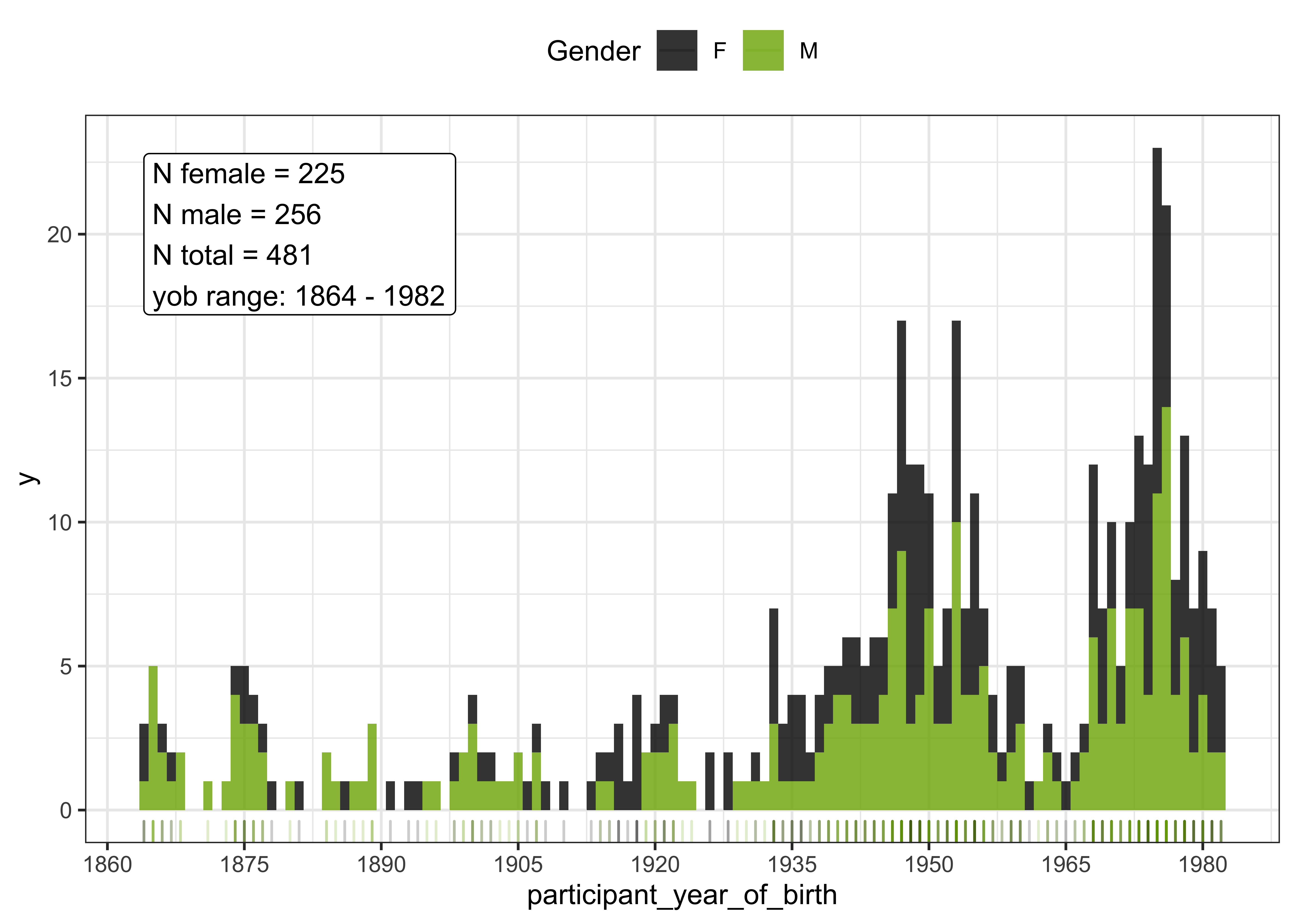

Below we provide summary information about each of the speakers token counts per vowel. This table comprises all speakers in the dataset and can be ordered and searched like a spreadsheet.

Normalisation

We will now normalise the raw F1 and F2 values.

Here, we introduce an adapted version of the Lobanov (1971) normalisation method, which we refer to as Lobanov 2.0. Explanations of the formula for each of the methods (Lobanov and Lobanov 2.0) are given below. Please refer to the paper for reasons why this adapted version was preferred to Lobanov’s original normalisation method.

Lobanov formula:

\[ \begin{equation} F_{lobanov_i} = \frac{(F_{raw_i}-\mu_{raw_i})}{\sigma_{raw_i}} \end{equation} \]

• \(i\) = either F1 or F2
• \(F_{lobanov_i}\) = the normalised value in \(i\)
• \(F_{raw_i}\) = the raw formant measurement value in \(i\)
• \(\mu_{raw_i}\) = the mean formant value calculated across all raw values in \(i\)
• \(\sigma_{raw_i}\) = the standard deviation calculated across all raw values in \(i\)

In plain English, the formula subtracts the mean formant value of a speaker from the raw individual formant value, then divides that by the standard deviation of the formant values.

e.g. if a speaker has a raw F1 of 400hz, a mean F1 of 500hz and a standard deviation of 70hz, this would give a Lobanov normalised value of (400-500)/70 = -1.43.

Lobanov 2.0 formula:

\[ \begin{equation} F_{lobanov2.0_i} = \frac{(F_{raw_i}-\mu_{(\mu_{vowel_1},\cdots,\mu_{vowel_n})})}{\sigma_{(\mu_{vowel_1},\cdots,\mu_{vowel_n})}} \end{equation} \]

• \(i\) = either F1 or F2
• \(F_{lobanov2.0_i}\) = the normalised value in \(i\)
• \(F_{raw_i}\) = the raw formant measurement value in \(i\)
• \(\mu_{(\mu_{vowel_1},\cdots,\mu_{vowel_n})}\) = the mean taken from the mean formant value calculated per vowel in \(i\)
• \(\sigma_{(\mu_{vowel_1},\cdots,\mu_{vowel_n})}\) = the standard deviation taken from the mean formant value calculated per vowel in \(i\)

In plain English, the formula subtracts the mean of means formant value of a speaker (calculated as the mean of means, where a mean for each vowel is calculated, then the mean taken of those means) from the raw individual formant value, then divides that by the standard deviation of the mean of mean values.

e.g. if a speaker has a raw F1 of 400hz, a mean of means F1 of 550hz and a standard deviation (for the mean of means) of 70hz, this would give a Lobanov 2.0 normalised value of (400-550)/70 = -2.14.

Implementation

The primary difference between the formula for this adapted version and Lobanov’s original formula, is that each of the vowels has a mean formant value calculated, then a mean of those means is taken as the mean in the formula. The motivation for doing this is that the data we are normalising contains speakers with varying numbers of tokens across the different vowels. Lobanov’s method is suited (and designed) based on balanced data, where an equal number of tokens per vowel are normalised.

When normalising with unbalanced numbers of tokens per vowel, the calculation of \(\mu_{raw_i}\) (the mean of all the raw formant values), can be skewed by tokens that have a much larger count in a certain vowel.

Therefore, we first calculate means for each of the individual vowels (per speaker, per formant), then calculate the mean based on those means. This approach allows for tokens in vowel categories to be weighted equally regardless of how many tokens there are, making the normalisation more reliable for this type of dataset.

For visualisation purposes, we plot the normalised values for F1 and F2 against each other in the plots below (Lobanov 2.0 is on the x axis and Lobanov on the y axis, with coloured lines representing each speaker, the black line represents where the values would be if they were equal, i.e. if Lobanov 2.0 = Lobanov)

#standard Lobanov normalisation - calculate means across all vowels per speaker
summary_vowels_all_lobanov <- vowels_all %>%
  group_by(Speaker) %>%
  dplyr::summarise(mean_F1_lobanov = mean(F1_50),
            mean_F2_lobanov = mean(F2_50),
            sd_F1_lobanov = sd(F1_50),
            sd_F2_lobanov = sd(F2_50),
            token_count = n())

#Lobanov 2.0 - calculate means per vowel and per speaker
summary_vowels_all <- vowels_all %>%
  group_by(Speaker, Vowel) %>%
  dplyr::summarise(mean_F1 = mean(F1_50),
            mean_F2 = mean(F2_50),
            sd_F1 = sd(F1_50),
            sd_F2 = sd(F2_50),
            token_count_vowel = n())

#get the mean_of_means and sd_of_means from the the speaker_summaries, this will give each speaker a mean caculated from the means across all vowels, as well as the standard deviation of the means
summary_mean_of_means <- summary_vowels_all %>%
  group_by(Speaker) %>%
  dplyr::summarise(mean_of_means_F1 = mean(mean_F1),
            mean_of_means_F2 = mean(mean_F2),
            sd_of_means_F1 = sd(mean_F1),
            sd_of_means_F2 = sd(mean_F2)
            )

#combine these values with the full raw dataset, then use these values to normalise the data with both the Lobanov and the Lobanov 2.0 method
vowels_all <- vowels_all %>%
  #add in the data
  left_join(., summary_mean_of_means) %>%
  left_join(., summary_vowels_all[, c("Speaker", "Vowel", "token_count_vowel")]) %>%
  left_join(., summary_vowels_all_lobanov) %>%
  #normalise the raw F1 and F2 values with Lobanov
  mutate(F1_lobanov = (F1_50 - mean_F1_lobanov)/sd_F1_lobanov,
         F2_lobanov = (F2_50 - mean_F2_lobanov)/sd_F2_lobanov,
  #normalise with Lobanov 2.0
         F1_lobanov_2.0 = (F1_50 - mean_of_means_F1)/sd_of_means_F1,
         F2_lobanov_2.0 = (F2_50 - mean_of_means_F2)/sd_of_means_F2) %>%
  #remove the variables that are not required
  dplyr::select(-(mean_of_means_F1:sd_of_means_F2), -(mean_F1_lobanov:sd_F2_lobanov))

#remove the previous summary data frames
rm(summary_vowels_all_lobanov, summary_vowels_all, summary_mean_of_means)

#inspect the relationship between the two normalised values
vowels_all %>%
  ggplot(aes(x = F1_lobanov_2.0, y = F1_lobanov, colour = Speaker)) +
  geom_smooth(method = "lm", size = 0.1, show.legend = FALSE) +
  geom_abline(slope=1, intercept=0) +
  theme_bw()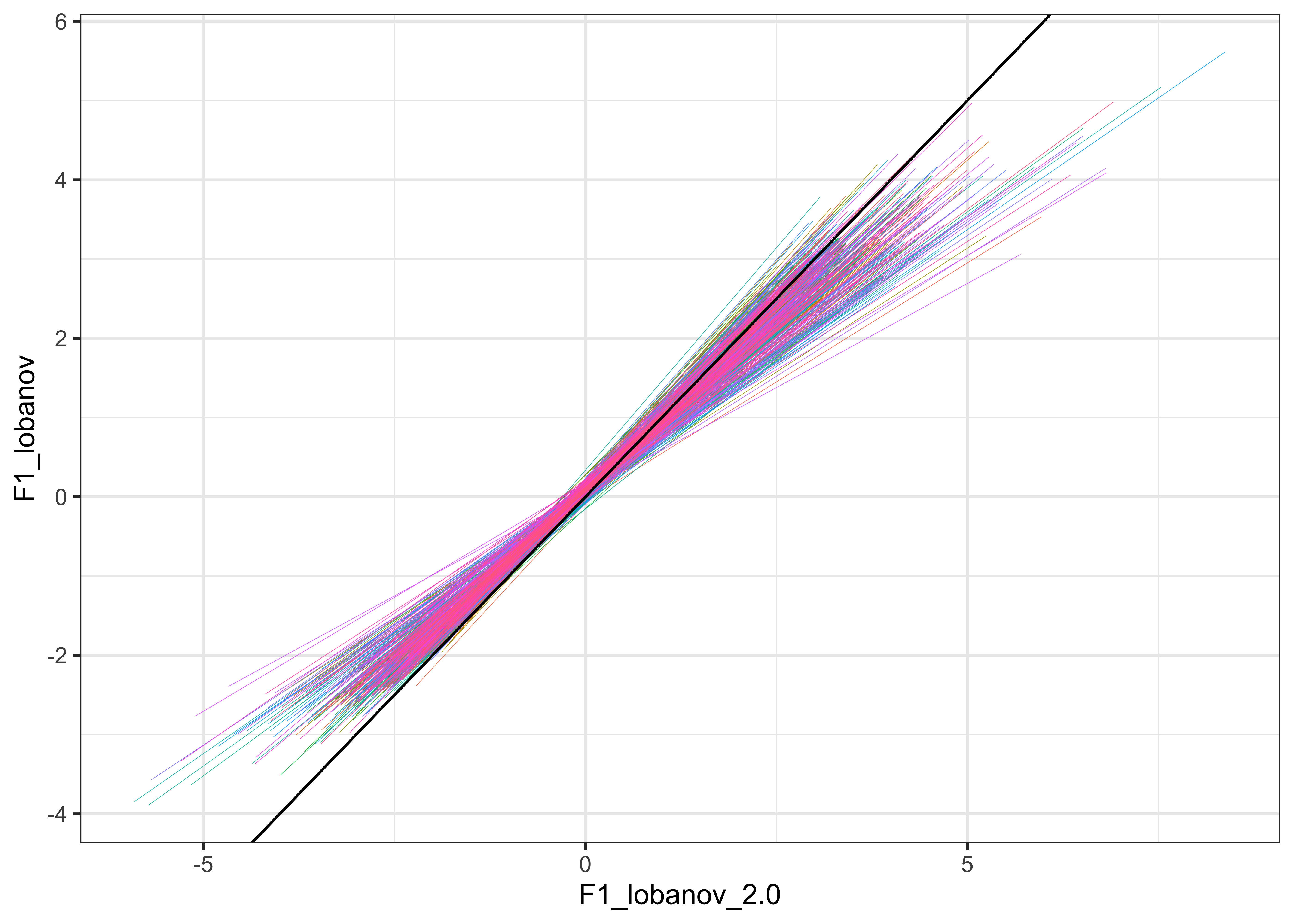

vowels_all %>%
  ggplot(aes(x = F2_lobanov_2.0, y = F2_lobanov, colour = Speaker)) +
  geom_smooth(method = "lm", size = 0.1, show.legend = FALSE) +
  geom_abline(slope=1, intercept=0) +
  theme_bw()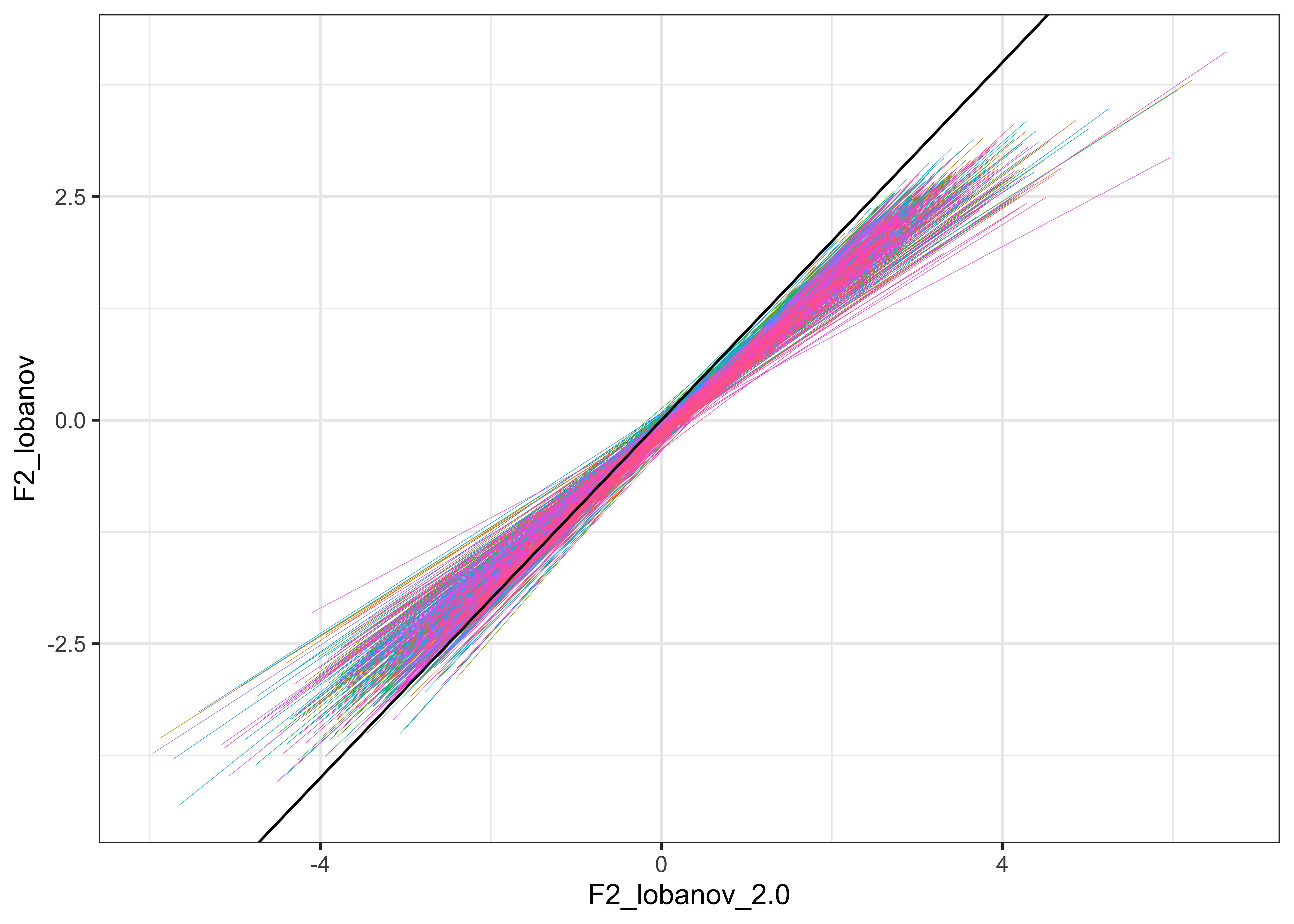

Make a plot for Figure 1 in the manuscript, of speakers born between 1900-1930. This will show the normalised vowel space and individual speaker means for the 10 vowels. There will also be ellipses to show the variation in the vowel productions and the black points indicate the individual vowel means, calculated across the sample of speakers.

#calculate individual speaker means for each vowel
vowel_means_example <- vowels_all %>%
  filter(participant_year_of_birth %in% c(1900:1930)) %>%
  group_by(Speaker, Vowel, Gender, participant_year_of_birth) %>%
  summarise(mean_F1 = mean(F1_lobanov_2.0),
            mean_F2 = mean(F2_lobanov_2.0))

vowel_means_example1 <- vowels_all %>%
  filter(participant_year_of_birth %in% c(1900:1930)) %>%
  group_by(Vowel) %>%
  summarise(mean_F1 = mean(F1_lobanov_2.0),
            mean_F2 = mean(F2_lobanov_2.0))

vowel_means_example_plot <- vowel_means_example %>%
  ggplot(aes(x = mean_F2, y = mean_F1, colour = Vowel)) +
  geom_point() +
  stat_ellipse(level = 0.67) +
  geom_label(data = vowel_means_example1, aes(label = Vowel)) +
  geom_point(data = vowel_means_example %>% filter(Speaker == "CC_f_326")) +
  geom_point(data = vowel_means_example %>% filter(Speaker == "CC_f_326"), colour = "black", size = 3, shape = 5, stroke = 2) +
  scale_x_reverse(name = "F2 (Normalised)", position = "top") +
  scale_y_reverse(name = "F1 (Normalised)", position = "right") +
  theme_bw() +
  theme(legend.position = "none")

vowel_means_example_plot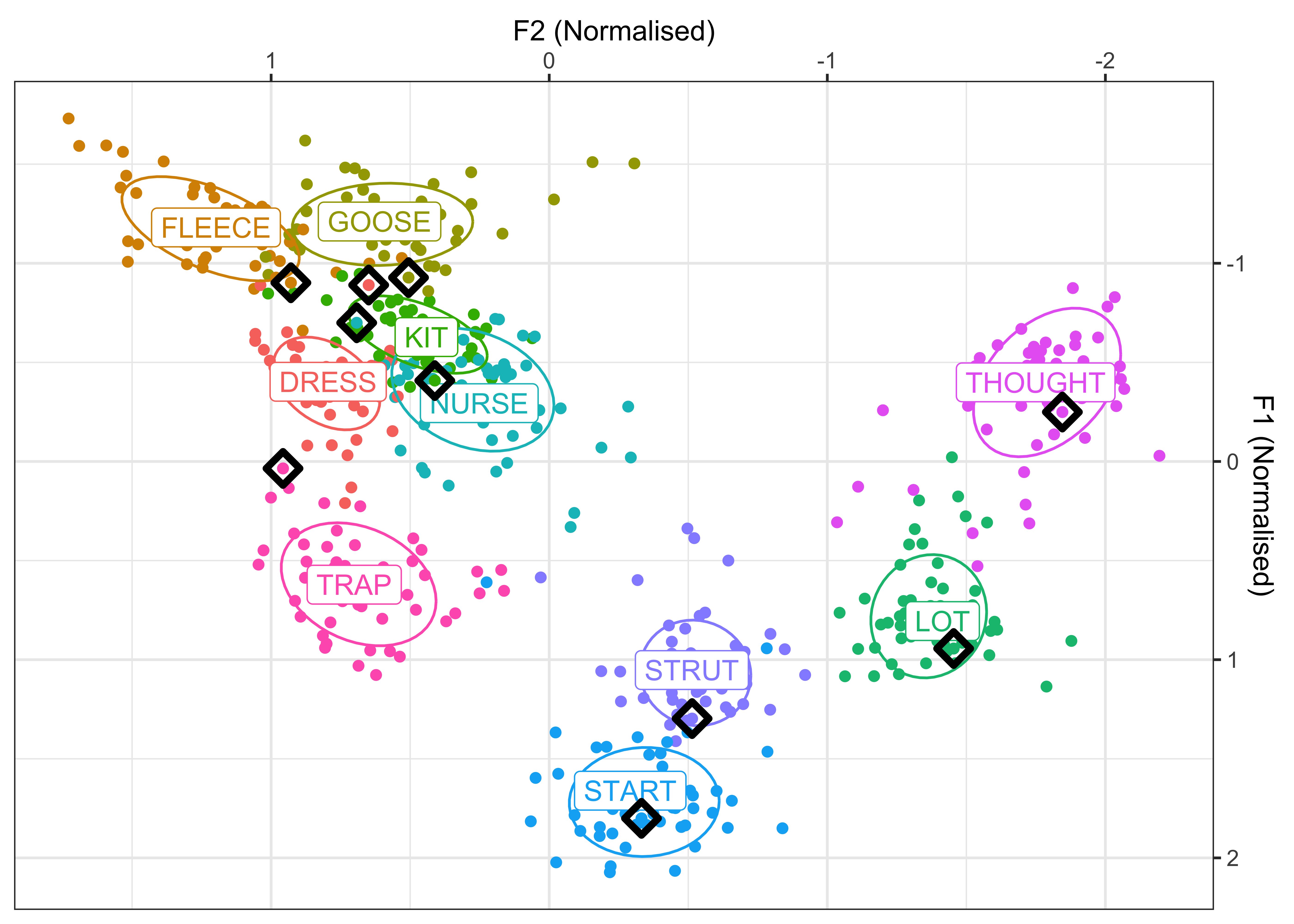

ggsave(plot = vowel_means_example_plot, filename = "Figures/vowel_means_example.png", dpi = 400)

GAMM modelling

In order to analyse co-variation in the dataset, we first must extract a measure of how the speakers vocalic variables differ from one another. To achieve this, we first run a series of Generalised Additive Mixed Models (GAMMs), from which we can extract the by-speaker random intercepts. This is done using the mgcv and itsadug packages, if you are unfamiliar with this form of analysis, see (Winter and Wieling, (2016))[https://academic.oup.com/jole/article/1/1/7/2281883] or (Sóskuthy, (2017))[https://arxiv.org/abs/1703.05339], for further information about why we chose the by-speaker intercepts, please refer to the manuscript or see Drager and Hay (2012)

In total there will be 20 separate models (10 vowels x 2 formants) that will be fitted, each of which we will extract the random intercepts from the random effect of Speaker, as well as the model summary.

Fitting procedure

Each of the models will use the data from one of the 10 vowels (in the Vowel variable) and will have either the F1_lobanov_2.0 or the F2_lobanov_2.0 variable as the dependent/predicted measure.

All models will be fit uniformly, i.e. with the same fixed and random effects structures.

The fixed effects are:

• An interaction between participant_year_of_birth and Gender

• participant_year_of_birth

• Gender

• Speech_rate

The random effects are:

• Speaker

• Word

The participant_year_of_birth variable is modeled with a smooth term with 10 knots, this is to account for the non-linear ‘wiggliness’ of the effect.

To run the models in an efficient way and store the by-speaker intercepts, we use a for loop to iterate through each of the vowels, extracting the intercepts from each model and adding them to a data frame.

A for loop works by iterating over each value in a series, here we will loop through each value in our Vowels variable and extract the relevant information.

e.g the for loop will start with DRESS, run the GAMM for F1, extract the by-speaker intercepts from that model, it will then run the GAMM for F2, extract the speaker intercepts from this model, then add the 2 sets of intercepts to a data frame (gam_intercepts.tmp). The loop will then move on to the next vowel, FLEECE and do exactly the same process. The loop will finish once all vowels have been ‘looped’ through.

This will result in a data frame comprising:

• 494 rows (one row per speaker)

• 1 column identifying the speaker name

• 20 additional columns identifying the variable being modeled (e.g. F1_DRESS), the numeric values here represent the by-speaker intercepts from that variable’s model

Note, this process takes several hours (six and half hours on my machine) to complete. The output has been stored in files in the GAMM_output folder, for quick reference. Please see those files or load them in to your R session for the rest of the analysis if you do not run the following code chunk.

The intercepts are saved as gamm_intercepts.csv, the model summaries can be found in the model_summaries sub-folder, where each model summary is stored as a .rds file, e.g. gam_summary_F1_DRESS.rds contains the model summary for F1_DRESS.

#update the Gender variable to allow for conrast coding
vowels_all$Gender <- as.ordered(vowels_all$Gender)
contrasts(vowels_all$Gender) <- "contr.treatment"

vowels_all <- vowels_all %>%
  arrange(as.character(Speaker))

#create a data frame to store the intercepts from the models, this will initially contain just the speaker names
gam_intercepts.tmp <- vowels_all %>%
  dplyr::select(Speaker) %>%
  distinct()

#loop through the vowels
cat(paste0("Start time:\n", format(Sys.time(), "%d %B %Y, %r\n")))

for (i in levels(factor(vowels_all$Vowel))) {
  
  #F1 modelling
  
  #run the mixed-effects model on the vowel, i.e. if i = FLEECE this will model F1 for FLEECE
  gam.F1 <- bam(F1_lobanov_2.0 ~
                  s(participant_year_of_birth, k=10, bs="ad", by=Gender) +
                  s(participant_year_of_birth, k=10, bs="ad") +
                  Gender +
                  s(Speech_rate) +
                  s(Speaker, bs="re") +
                  s(Word, bs="re"),
                data=vowels_all %>% filter(Vowel == i),
                discrete=T, nthreads=2)
  
  #extract the speaker intercepts from the model and store them in a temporary data frame
  gam.F1.intercepts.tmp <- as.data.frame(get_random(gam.F1)$`s(Speaker)`)
  
  #assign the model to an object
  assign(paste0("gam_F1_", i), gam.F1)
  
  #save the model summary
  saveRDS(gam.F1, file = paste0("/Users/james/Documents/GitHub/model_summaries/gam_F1_", i, ".rds"))
  
  cat(paste0("F1_", i, ": ", format(Sys.time(), "%d %B %Y, %r"), " ✅\n")) #print the vowel the loop is up to for F1, as well as the start time for the model
  
  #F2 modelling
  
  #run the mixed-effects model on the vowel, i.e. if i = FLEECE this will model F2 for FLEECE
  gam.F2 <- bam(F2_lobanov_2.0 ~
                  s(participant_year_of_birth, k=10, bs="ad", by=Gender) +
                  s(participant_year_of_birth, k=10, bs="ad") +
                  Gender +
                  s(Speech_rate) +
                  s(Speaker, bs="re") +
                  s(Word, bs="re"),
                data=vowels_all %>% filter(Vowel == i),
                discrete=T, nthreads=2)
  
  #extract the speaker intercepts again, storing them in a separate data frame
  gam.F2.intercepts.tmp <- as.data.frame(get_random(gam.F2)$`s(Speaker)`)
  
  #assign the model to an object
  assign(paste0("gam_F2_", i), gam.F2)
  
  #save the model summary
  saveRDS(gam.F2, file = paste0("/Users/james/Documents/GitHub/model_summaries/gam_F2_", i, ".rds"))

  #rename the variables so it clear which one has F1/F2, i.e. this will give F1_FLEECE, F2_FLEECE
  names(gam.F1.intercepts.tmp) <- paste0("F1_", i)
  names(gam.F2.intercepts.tmp) <- paste0("F2_", i)
  
  #combine the intercepts for F1 and F2 and store them in the intercepts.tmp_stress data frame
  gam_intercepts.tmp <- cbind(gam_intercepts.tmp, gam.F1.intercepts.tmp, gam.F2.intercepts.tmp)
  
  cat(paste0("F2_", i, ": ", format(Sys.time(), "%d %B %Y, %r"), " ✅\n")) #print the vowel the loop is up to for F2 , as well as the start time for the model
}

#save the intercepts as a .csv file
write.csv(gam_intercepts.tmp, "Data/gam_intercepts_tmp_new.csv", row.names = FALSE)

Read in pre-run model results

In order to save time running through the GAMM modelling chunk above, the results have been stored in the repository for quick loading. The below code will load the files in to your R session.

#load in model intercepts
gam_intercepts.tmp <- read.csv("Data/gam_intercepts_tmp_new.csv")

#make vector containing all .rds filenames from model_summaries folder
model_summary_files = list.files(pattern="*.rds", path = "/Users/james/Documents/GitHub/model_summaries")

#load each of the files with for loop
for (i in model_summary_files) {
  cat(paste0(i, ": ", format(Sys.time(), "%d %B %Y, %r"), " ✅\n")) 
  assign(gsub(".rds", "", i), readRDS(paste0("/Users/james/Documents/GitHub/model_summaries/", i)))
}

Understanding the intercepts

In order to better understand these intercepts and how they represent each speaker’s position in relation to the population, it can be helpful to visualise the speaker intercepts in relation to the vowel space.

We interpret the speaker intercepts in terms of how advanced the vowel productions are in relation to other speakers with similar fixed-effects - in other words, if a speaker has a large positive intercept from a model (with a fixed-effects structure as that used in our above modelling procedure), this would indicate that the speaker is producing formant values that are typically larger than other speakers with similar fixed-effects values, e.g. year of birth, gender etc. Likewise, if the intercept is negative, this would indicate that their F values are smaller, the closer the intercept is to 0, the more typical the speaker is (taking into account the fixed-effects).

To demonstrate this, we will visualise the change in F1 for three vowels, known to have undergone rapid change in New Zealand English (TRAP, DRESS and KIT). We will plot the participant year of birth on the x axis and normalised F1 on the y axis (reverse scaled to match normal vowel plot conventions). To highlight the change in the three vowels over time, we will also fit a smooth and plot the mean F1 values of each speaker for each of the vowels. Finally, we will highlight 4 speakers who all have intercepts that indicate that they are advanced in these vowel changes, i.e. have negative intercepts (smaller F1) for TRAP and DRESS, but positive intercepts (larger F1) for KIT.

The first chunk calculates mean F1 values / speaker and merges this data with the speaker intercepts from the GAMMs.

The second chunk extracts predictions from the GAMMs for plotting smooths over year of birth. (This code block produces plots that are not included in the RMarkdown output).

vowels_to_plot <- c("KIT", "DRESS", "TRAP")

pred_table <- function (Vowel) {
  mod_name <- paste0("gam_F1_", Vowel)
  return(cbind(Vowel, 
               plot_smooth(get(mod_name), view="participant_year_of_birth", 
                           rm.ranef=T, rug=F, n.grid=119)$fv)
  )
}

gamm_preds_to_plot <- lapply(vowels_to_plot, pred_table) %>%
  do.call(rbind, .)

saveRDS(gamm_preds_to_plot, "Data/Models/gamm_preds_to_plot.rds")

gamm_preds_to_plot <- readRDS("Data/Models/gamm_preds_to_plot.rds")

We now plot the data.

#make a long version of the intercepts
gam_intercepts.tmp_long <- gam_intercepts.tmp %>%
  pivot_longer(F1_DRESS:F2_TRAP, names_to = "Vowel_formant", values_to = "Intercept") %>%
  mutate(Formant = substr(Vowel_formant, 1, 2),
         Vowel = substr(Vowel_formant, 4, max(nchar(Vowel_formant)))) %>%
  left_join(vowels_all %>%
  select(Speaker, participant_year_of_birth) %>% distinct()) %>%
  left_join(gamm_preds_to_plot %>% mutate(Formant = "F1") %>% select(participant_year_of_birth, Vowel, Formant, fit, ll, ul))

speakers1 <- gam_intercepts.tmp_long %>%
  filter(Vowel_formant %in% c("F1_KIT", "F1_DRESS", "F1_TRAP")) %>%
  ungroup() %>%
  arrange(participant_year_of_birth) %>%
  filter(Speaker %in% c("MU_m_348", "IA_f_341", "CC_m_167", "CC_f_297")) %>%
  mutate(letters = c(rep("A", 3), rep("B", 3), rep("C", 3), rep("D", 3)),
         speakers1 = paste0(letters, " (", round(Intercept, 2), ")"))

F1_speaker_intercepts <- gam_intercepts.tmp_long %>%
  filter(Vowel %in% c("KIT", "DRESS", "TRAP"),
         Formant == "F1") %>% #choose the vowels
  mutate(Vowel = factor(Vowel, levels = c("TRAP", "DRESS", "KIT"))) %>% #order the vowels
  ggplot(aes(x = participant_year_of_birth, y = fit, colour = Vowel, fill = Vowel)) +
  geom_point(aes(x = participant_year_of_birth, y = fit + Intercept), size = 1, alpha = 0.2) +
  geom_line() +
  geom_ribbon(aes(ymin=ll, ymax=ul), colour = NA, alpha=0.2) +
  geom_point(data = speakers1 %>% mutate(fit = ifelse(speakers1 %in% c("D (-0.36)"), fit - 0.05, fit)), aes(x = participant_year_of_birth, y = fit + Intercept), size = 4) +
  geom_label(data = speakers1 %>% mutate(fit = ifelse(speakers1 %in% c("B (0.23)"), fit - 0.1, fit), fit = ifelse(speakers1 %in% c("D (-0.36)"), fit - 0.1, fit)), aes(x = participant_year_of_birth - 1, y = fit + Intercept, label = speakers1), fill = "white", alpha = 0.5, hjust = 1, show.legend = FALSE) +
  scale_y_reverse() +
  scale_colour_manual(values=c("#E69F00", "#56B4E9", "#009E73")) +
  scale_fill_manual(values=c("#E69F00", "#56B4E9", "#009E73")) +
  xlab("Participant year of birth") + #x axis title
  ylab("Normalised F1 (Lobanov 2.0)") + #y axis title
  theme_bw() + #general aesthetics
  theme(legend.position = c(0.8, 0.1), #legend position
        legend.direction = "horizontal",
        legend.background = element_rect(colour = "black"),
        axis.text = element_text(size = 14), #text size
        axis.title = element_text(face = "bold", size = 14), #axis text aesthetics
        legend.title = element_blank(), #legend title text size
        legend.text = element_text(size = 14)) #legend text size
 
F1_speaker_intercepts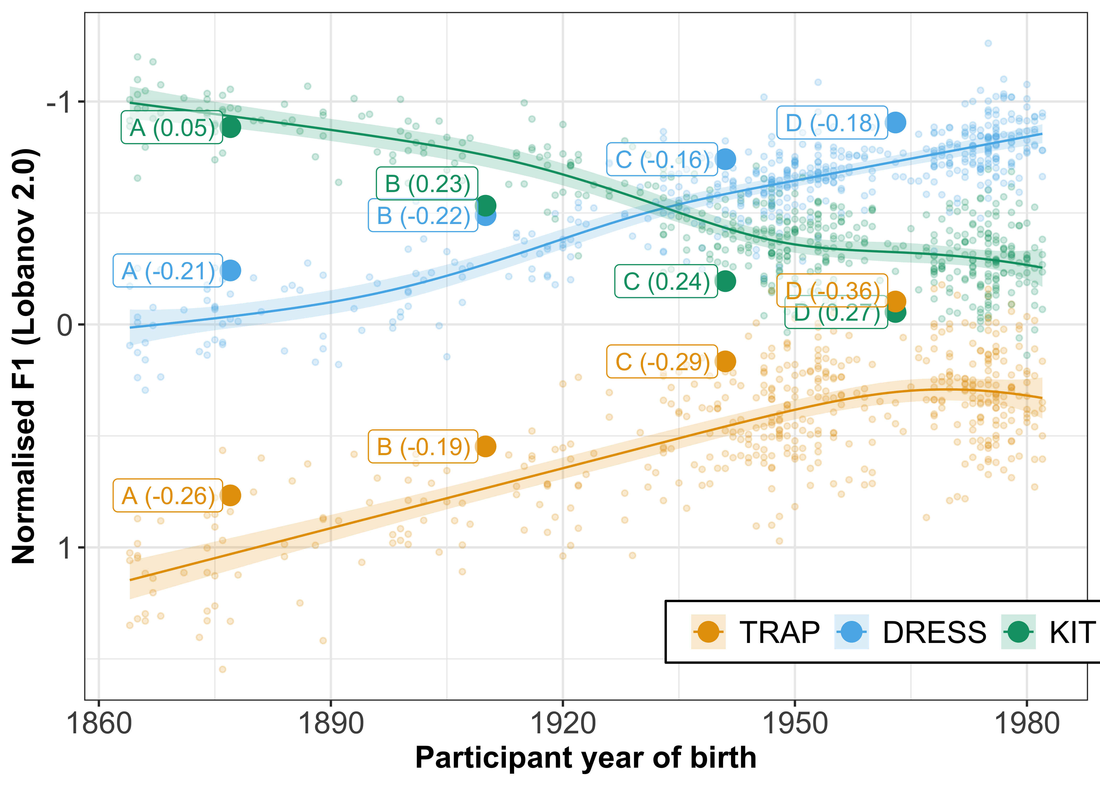

ggsave(plot = F1_speaker_intercepts, filename = "Figures/F1_speaker_intercepts.png", width = 10, height = 5, dpi = 400)

#clean up
rm(speakers, speakers1, F1_speaker_intercepts)

Visualisation of intercept correlations

Understanding how the intercepts may be correlated to each other is an important first step to how they relate to each other. However, simply using correlations to gain a full understanding of how the covariation is operating, may not be sufficient. We present below an initial outline of the correlations between the intercepts.

1. Checking the distribution of the intercepts

gam_intercepts.tmp %>%
  select(-1) %>%
  pivot_longer(cols = 1:20, names_to = "variable", values_to = "intercept") %>%
  ggplot(aes(x = intercept, y = ..density..)) +
  geom_histogram(bins = 500) +
  geom_density(outline.type = "upper", colour = "red", bw = "SJ") +
  facet_wrap(~variable) +
  theme_bw()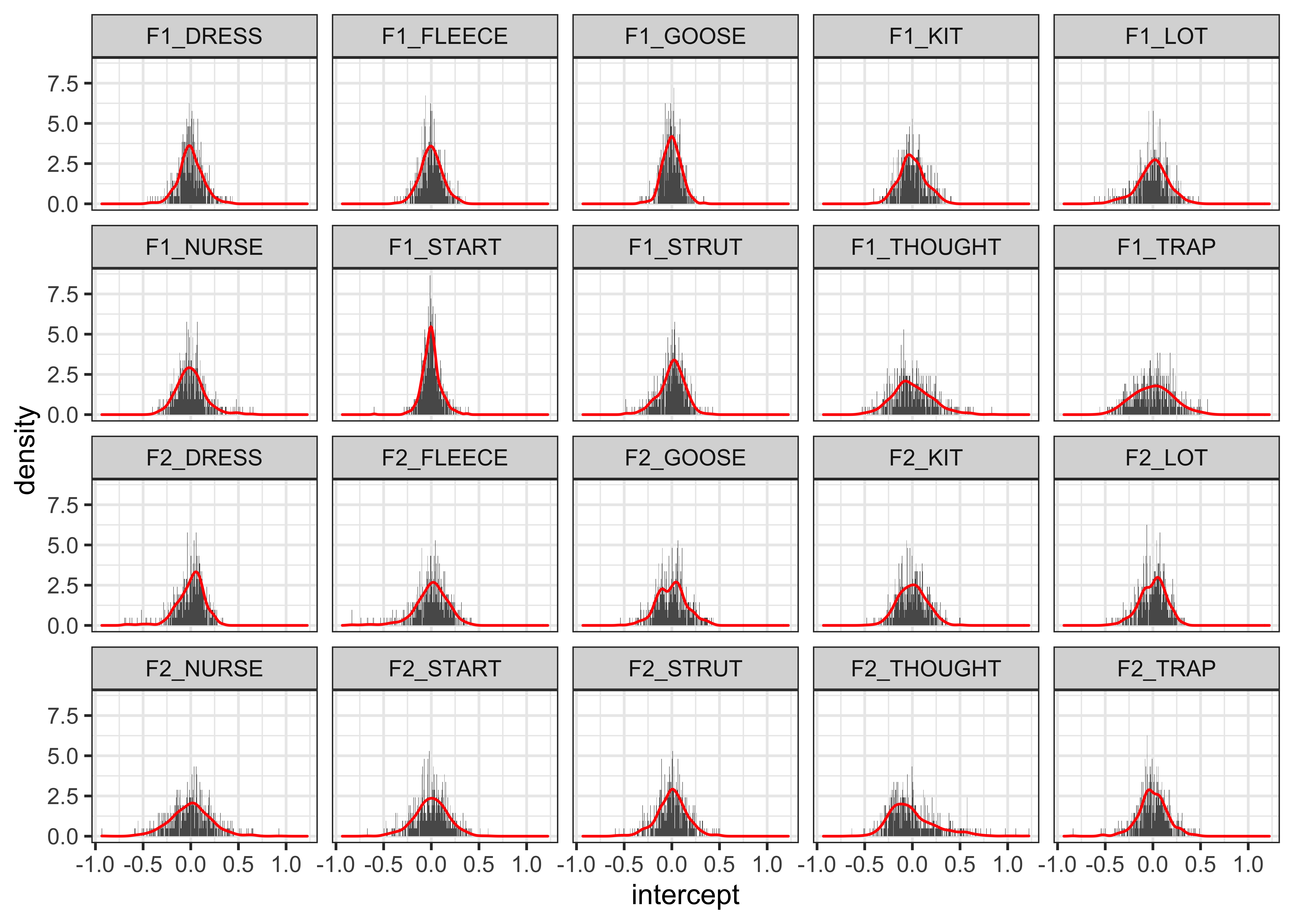

2. The correlations themselves

intercepts_cor <- cor(gam_intercepts.tmp[-1] %>%
             select(starts_with("F1"), starts_with("F2")))

datatable(intercepts_cor) %>%
  formatRound(columns = 1:20)

3. A chord plot that visualises the correlations. This plot will give a more simplified representation of the above plot, it connects each of the variables to all the other variables via chords. The black chords indicate a positive correlation, whereas a red chord represents a negative correlation. The size and transparency of the chord indicates the strength of the correlation, with darker wider chords being used for the strongest correlations

The code below adapts the code used in Zuguang Gu’s tutorial (see http://jokergoo.github.io/blog/html/large_matrix_circular.html)

mat <- cor(gam_intercepts.tmp[-1] %>%
             select(starts_with("F2"), starts_with("F1")))

diag(mat) = 0
mat[lower.tri(mat)] = 0
n = nrow(mat)
rn = rownames(mat)

group_size = c(rep(1, 20))
gl = lapply(1:20, function(i) {
    rownames(mat)[sum(group_size[seq_len(i-1)]) + 1:group_size[i]]
})
names(gl) = names(mat)

group_color = structure(circlize::rand_color(20), names = names(gl))
n_group = length(gl)

col_fun = colorRamp2(c(-1, 0, 1), c("red", "transparent", "black"), transparency = 0.1)

par(mfrow=c(1,3))

# < |0.2|
mat1 <- ifelse(mat < 0.2 & mat > -0.2, mat, 0)

col2 <- col_fun(mat1)
col2 <- ifelse(col2 == "#FFFFFFE6", NA, col2)

chordDiagram(mat, col = col2, grid.col = NA, grid.border = "black", 
                      annotationTrack = "grid", link.largest.ontop = TRUE,
                      preAllocateTracks = list(
                        list(track.height = 0.02)
                      )
)

title("r < |0.2|", cex.main = 2.5, line = -2)

circos.trackPlotRegion(track.index = 2, panel.fun = function(x, y) {
  xlim = get.cell.meta.data("xlim")
  ylim = get.cell.meta.data("ylim")
  sector.index = get.cell.meta.data("sector.index")
  circos.text(mean(xlim), mean(ylim), sector.index, col = "black", cex = 0.6, 
              facing = "inside", niceFacing = TRUE)
}, bg.border = NA)

# |0.2-0.3|
mat1 <- ifelse(mat > 0.3 | mat < -0.3, 0, mat)
mat1 <- ifelse(mat1 < 0.2 & mat1 > -0.2, 0, mat1)

col2 <- col_fun(mat1)
col2 <- ifelse(col2 == "#FFFFFFE6", NA, col2)

chordDiagram(mat, col = col2, grid.col = NA, grid.border = "black", 
             annotationTrack = "grid", link.largest.ontop = TRUE,
             preAllocateTracks = list(
               list(track.height = 0.02)
             )
)

title("r between |0.2 - 0.3|", cex.main = 2.5, line = -2)

circos.trackPlotRegion(track.index = 2, panel.fun = function(x, y) {
  xlim = get.cell.meta.data("xlim")
  ylim = get.cell.meta.data("ylim")
  sector.index = get.cell.meta.data("sector.index")
  circos.text(mean(xlim), mean(ylim), sector.index, col = "black", cex = 0.6, 
              facing = "inside", niceFacing = TRUE)
}, bg.border = NA)

# > |0.3|
mat1 <- ifelse(mat > 0.3 | mat < -0.3, mat, 0)

col2 <- col_fun(mat1)
col2 <- ifelse(col2 == "#FFFFFFE6", NA, col2)

chordDiagram(mat, col = col2, grid.col = NA, grid.border = "black", 
             annotationTrack = "grid", link.largest.ontop = TRUE,
             preAllocateTracks = list(
               list(track.height = 0.02)
             )
)

title("r between |0.3 - 0.6|", cex.main = 2.5, line = -2)

circos.trackPlotRegion(track.index = 2, panel.fun = function(x, y) {
  xlim = get.cell.meta.data("xlim")
  ylim = get.cell.meta.data("ylim")
  sector.index = get.cell.meta.data("sector.index")
  circos.text(mean(xlim), mean(ylim), sector.index, col = "black", cex = 0.6, 
              facing = "inside", niceFacing = TRUE)
}, bg.border = NA)

4. Heat map of the correlations

cors <- function(df) { 
   # turn all three matrices (r, n, and P into a data frame)
   M <- Hmisc::rcorr(as.matrix(df))
   # return the three data frames in a list return(Mdf)
   Mdf <- map(M, ~data.frame(.x))
}

formatted_cors <- function(df){
 cors(df) %>%
 map(~rownames_to_column(.x, var="measure1")) %>%
 map(~pivot_longer(.x, -measure1, "measure2")) %>% 
 bind_rows(.id = "id") %>%
 pivot_wider(names_from = id, values_from = value) %>%
 mutate(sig_p = ifelse(P < .05, T, F), p_if_sig = ifelse(P <.05, P, NA), r_if_sig = ifelse(P <.05, r, NA))
}

formatted_cors(gam_intercepts.tmp[-1]) %>%
 ggplot(aes(x = measure1, y = measure2, fill = r, label=round(r_if_sig,2))) +
 geom_tile() +
 geom_text(aes(size = abs(r_if_sig)), show.legend = FALSE) +
 labs(x = NULL, y = NULL, fill = "Pearson's Correlation") +
 # map a red, white and blue color scale to correspond to -1:1 sequential gradient
 scale_fill_gradient2(mid="#FBFEF9",low="#0C6291",high="#A63446", limits=c(-1,1)) +
 theme_classic() +
 # remove excess space on x and y axes
 scale_x_discrete(expand=c(0,0)) +
 scale_y_discrete(expand=c(0,0)) +
 # change global font to roboto
 theme(axis.text = element_text(size = 20, face = "bold"),
       axis.text.x = element_text(angle = 90, hjust = 1),
       legend.position = "top",
       legend.key.width = unit(2, "cm"),
       legend.title = element_text(size = 20),
       legend.text = element_text(size = 20)) +
  guides(fill = guide_colourbar(title.position = "top"))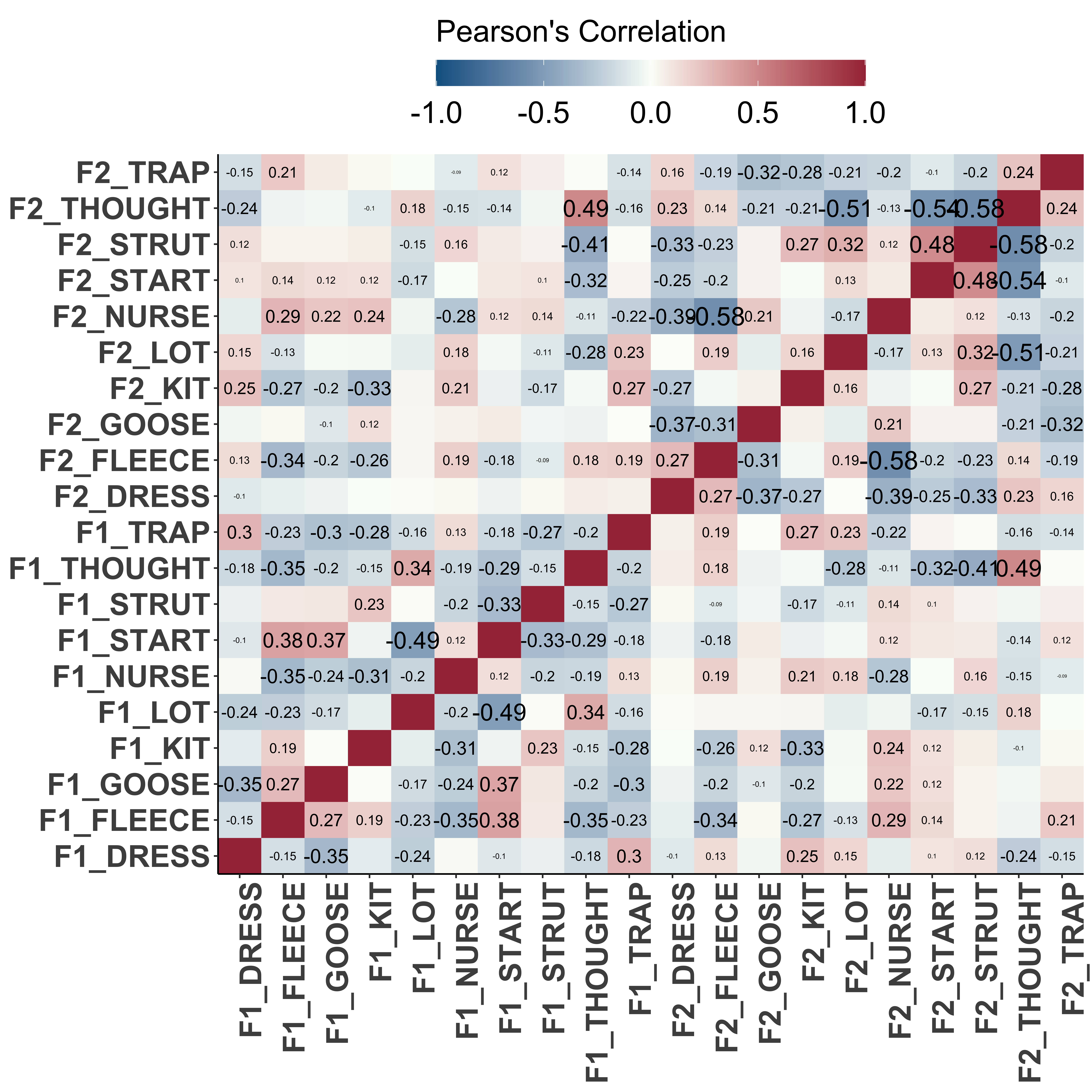

5. Table of correlations with significance

formatted_cors(gam_intercepts.tmp[-1]) %>%
  filter(r != 1) %>%
  mutate(absolute_r = abs(r)) %>%
  arrange(-absolute_r) %>%
  group_by(r) %>%
  mutate(id = row_number()) %>%
  ungroup() %>%
  filter(id == 1) %>%
  datatable() %>%
  formatRound(c("r", "r_if_sig", "P", "p_if_sig", "absolute_r"), 3)

6. Permutation of correlations

This is the plot we include in the manuscript.

We show the distribution of correlation co-efficients across the intercepts (plotted in red), highlighting that there are a range of positive/negative correlations, some stronger than others.

We permute the correlations 100 times (which is a process of shuffling the values around to remove any underlying structure). This distribution is plotted in blue and shows that the random correlations are generally between |1.5|. Thus, the correlations in the ONZE dataset are likely to represent actual co-variation between the variables.

correlations_permuted <- gam_intercepts.tmp[-1] %>%
  formatted_cors(.) %>%
  mutate(intercepts = "ONZE")

for (i in 1:100) {
  permuted <- formatted_cors(apply(gam_intercepts.tmp[-1], 2L, sample)) %>% mutate(intercepts = i)
  
  correlations_permuted <<- rbind(correlations_permuted, permuted)
}

correlations_permuted <- correlations_permuted %>%
  mutate(Data = ifelse(intercepts == "ONZE", "ONZE", "Permuted")) %>%
  filter(r < 1)

correlations_permuted_plot <- ggplot(correlations_permuted, aes(x = r, y = ..density.., colour = Data, group = intercepts)) +
  # geom_histogram(alpha = 0.1, bins = 481) +
  geom_line(aes(x = r, y = P),size = 0) +
  geom_density(aes(colour = Data), adjust = 0.2, size = 0.01, alpha = 1, show.legend = FALSE) +
  geom_density(data = correlations_permuted %>% filter(intercepts == "ONZE"), adjust = 0.2, colour = "#F8766D", size = 1, show.legend = FALSE) +
  scale_x_continuous(limits = c(-0.6, 0.6)) +
  xlab("Pearson's correlation co-efficient (r)") +
  # facet_grid(~intercepts) +
  theme_bw() +
  theme(legend.position = "top",
        legend.title = element_blank(),
        axis.title = element_text(size = 14, face = "bold"),
        legend.text = element_text(size = 14, face = "bold")) +
  guides(colour = guide_legend(override.aes = list(size=1)))

positive_correlations <- ggplot(correlations_permuted, aes(x = r, y = ..density.., colour = Data, group = intercepts)) +
  geom_density(size = 0) +
  annotate("rect", xmin = -1, xmax = 0.57, ymin = 2, ymax = 10, fill = "cornsilk", colour = "black") +
  annotate("text", label = "Top 5 positive correlations:", fontface = 2, x = -0.95, y = 9.5, hjust = 0, vjust = 1, size = 4) +
  annotate("text", label = "F1 THOUGHT ~ F2 THOUGHT (r = .49)\nF2 START ~ F2 STRUT (r = .48)\nF1 FLEECE ~ F1 START (r = .38)\nF1 GOOSE ~ F1 START (r = 0.37)\nF1 LOT ~ F1 THOUGHT (r = 0.34)", x = -0.95, y = 7.5, hjust = 0, vjust = 1, size = 4) +
  theme_nothing()

negative_correlations <- ggplot(correlations_permuted, aes(x = r, y = ..density.., colour = Data, group = intercepts)) +
  geom_density(size = 0) +
  annotate("rect", xmin = -1, xmax = 0.57, ymin = 2, ymax = 10, fill = "cornsilk", colour = "black") +
  annotate("text", label = "Top 5 negative correlations:", fontface = 2, x = -0.95, y = 9.5, hjust = 0, vjust = 1, size = 4) +
  annotate("text", label = "F2 STRUT ~ F2 THOUGHT (r = -.58)\nF2 FLEECE ~ F2 NURSE (r = -.58)\nF2 START ~ F2 THOUGHT (r = -.54)\nF2 LOT ~ F2 THOUGHT (r = -.51)\nF1 LOT ~ F1 START (r = -.49)", x = -0.95, y = 7.5, hjust = 0, vjust = 1, size = 4) +
  theme_nothing()

correlations_permuted_plot1 <- plot_grid(correlations_permuted_plot, plot_grid(negative_correlations, positive_correlations, nrow = 1, ncol = 2), rel_heights = c(0.8, 0.4),  nrow = 2, ncol = 1)

correlations_permuted_plot1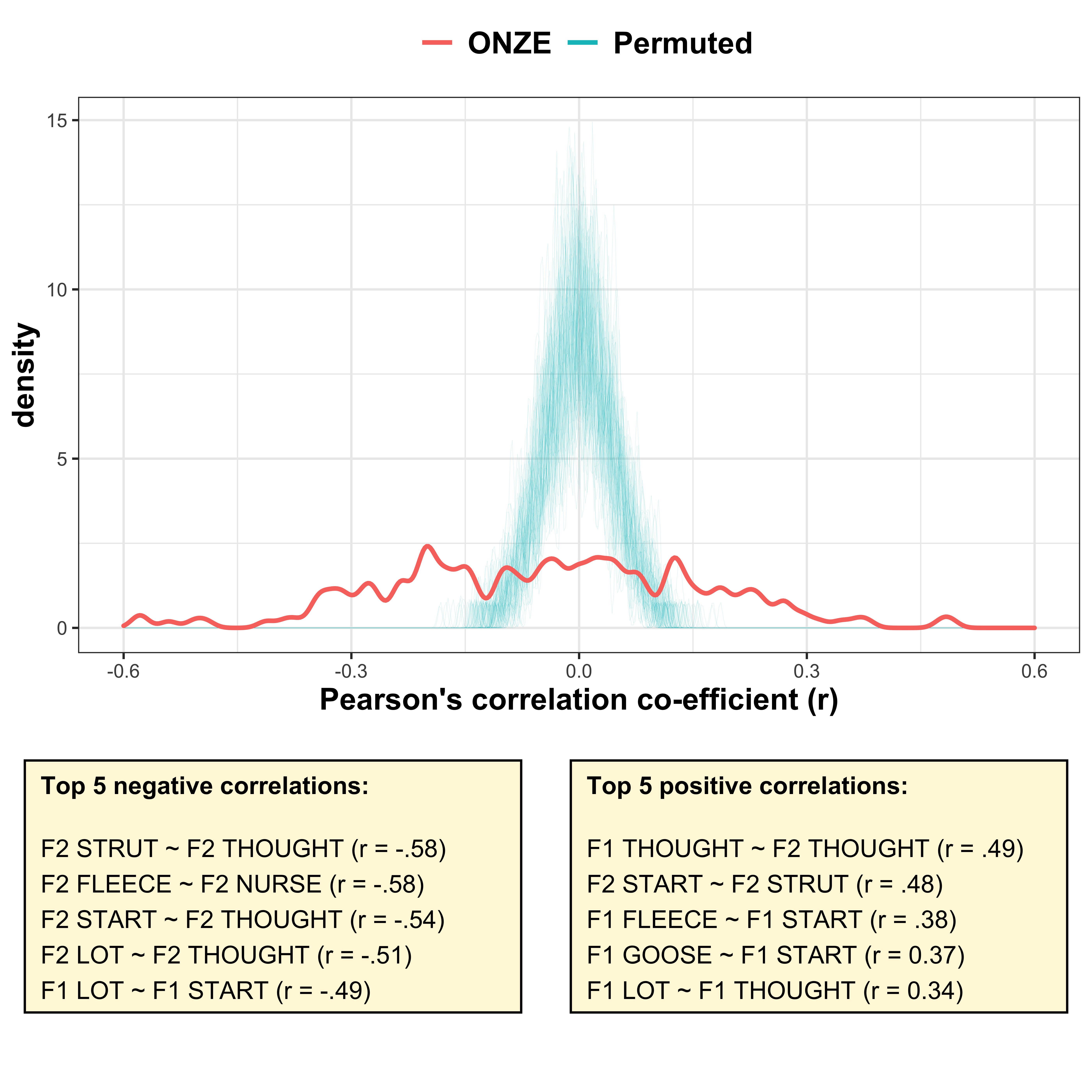

ggsave(plot = correlations_permuted_plot1, filename = "Figures/correlations_permuted_plot.png", width = 7, height = 7, dpi = 400)

Principal Components Analysis (PCA)

In the following section we will run a PCA on the gam_intercepts.tmp data frame, i.e. the by-speaker intercepts from each of the 20 GAMMs.

PCA offers a neat analysis solution to assessing whether there is underlying structure in the dataset, by highlighting which variables co-vary together - these are called principal components (PCs). Moreover, it also allows us to explore the data at the by-speaker level, providing us with insights into who is on the margins of these PCs.

Running the PCA

#run the PCA on the intercepts data frame, note the intercepts are in columns 2:21 as column 1 is the speaker name
intercepts.pca <- princomp(gam_intercepts.tmp[, 2:ncol(gam_intercepts.tmp)],cor=TRUE)

#print a summary of the PCA, this will give the variance explained by each PC
summary(intercepts.pca)

## Importance of components:
##                           Comp.1    Comp.2    Comp.3     Comp.4     Comp.5
## Standard deviation     1.8568236 1.7761654 1.4218609 1.27801065 1.11351321
## Proportion of Variance 0.1723897 0.1577382 0.1010844 0.08166556 0.06199558
## Cumulative Proportion  0.1723897 0.3301279 0.4312123 0.51287786 0.57487344
##                           Comp.6     Comp.7     Comp.8     Comp.9    Comp.10
## Standard deviation     1.0424970 1.00352469 0.95546926 0.90696297 0.87916274
## Proportion of Variance 0.0543400 0.05035309 0.04564608 0.04112909 0.03864636
## Cumulative Proportion  0.6292134 0.67956653 0.72521261 0.76634170 0.80498805
##                           Comp.11    Comp.12    Comp.13    Comp.14    Comp.15
## Standard deviation     0.80953378 0.77331213 0.73748412 0.72788478 0.67193061
## Proportion of Variance 0.03276725 0.02990058 0.02719414 0.02649081 0.02257454
## Cumulative Proportion  0.83775530 0.86765588 0.89485002 0.92134084 0.94391538
##                           Comp.16    Comp.17    Comp.18     Comp.19    Comp.20
## Standard deviation     0.61321385 0.55845231 0.47851298 0.372962769 0.25635209
## Proportion of Variance 0.01880156 0.01559345 0.01144873 0.006955061 0.00328582
## Cumulative Proportion  0.96271694 0.97831039 0.98975912 0.996714180 1.00000000

#view eigen values, this will visualise the variance explained by each PC
fviz_eig(intercepts.pca, addlabels = TRUE)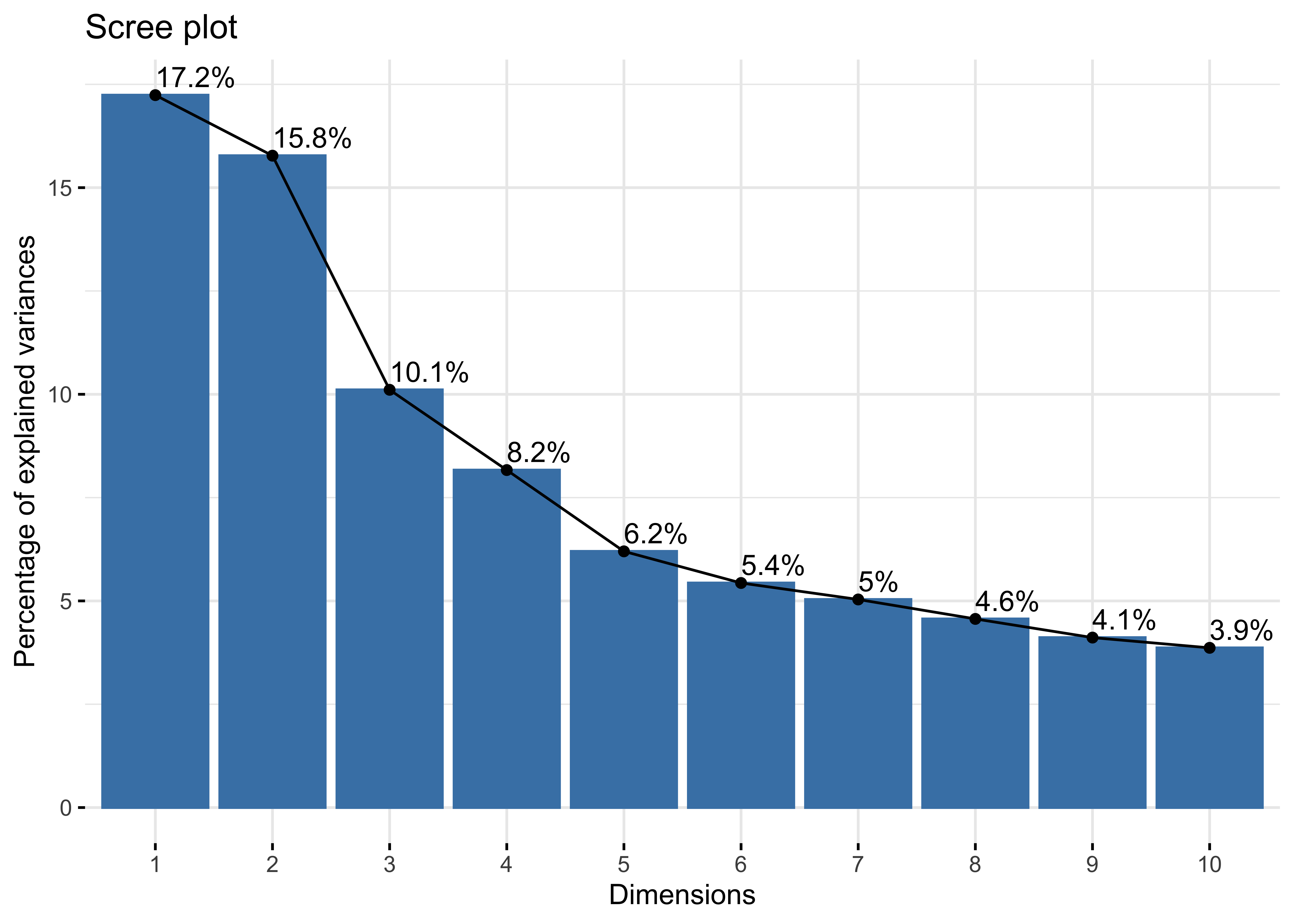

#create objects containing the loadings for each of the 3 main PCs
PC1_loadings <- intercepts.pca$loadings[,1]
PC2_loadings <- intercepts.pca$loadings[,2]
PC3_loadings <- intercepts.pca$loadings[,3]

We can also permute the data again and run the PCA to compare how the ONZE intercepts compare to permuted intercepts. We can see a clear difference between the two data sets. The 4th PC from the ONZE intercepts does appear to explain more variance than the permuted intercepts, but we chose to focus on the first 3 PCs as each explains > 10% of the variance in the analysis (dashed horizontal line), which is commonly taken as a threshold for meaningfully interpretable PCs.

PCA_variance_permuted <- get_eigenvalue(intercepts.pca)[1:10, 2] %>%
  data.frame() %>%
  rename(Variance = 1) %>%
  mutate(PC = paste0(1:10),
         Permutation = "ONZE",
         Data = "ONZE") %>%
  select(PC, Variance, Permutation, Data)

for (i in 1:100) {
  permuted <- apply(gam_intercepts.tmp[-1], 2L, sample)
  
  permuted_pca <- princomp(permuted, cor = TRUE)
  
  PCA_variance <- get_eigenvalue(permuted_pca)[1:10, 2] %>%
  data.frame() %>%
  rename(Variance = 1) %>%
  mutate(PC = paste0(1:10),
         Permutation = i,
         Data = "Permuted") %>%
  select(PC, Variance, Permutation, Data)
  
  PCA_variance_permuted <<- rbind(PCA_variance_permuted, PCA_variance)
}

PCA_variance_permuted_plot <- PCA_variance_permuted %>%
  group_by(Data, PC) %>%
  summarise(mean_variance = mean(Variance),
            sd = sd(Variance)) %>%
  arrange(PC) %>%
  mutate(PC = factor(PC, levels = c(1, 2, 3, 4, 5, 6, 7, 8, 9, 10)),
         sd = ifelse(is.na(sd), 0, sd)) %>%
  ggplot(aes(x = PC, y = mean_variance, colour = Data, group = Data)) +
  geom_point(data = PCA_variance_permuted %>%
  mutate(PC = factor(PC, levels = c(1, 2, 3, 4, 5, 6, 7, 8, 9, 10))), aes(x = PC, y = Variance), size = 0.1, alpha = 0.1) +
  geom_errorbar(aes(ymin=mean_variance-sd, ymax=mean_variance+sd), width=.1, position=position_dodge(0.1)) +
  geom_line() +
  geom_point() +
  geom_hline(yintercept = 10, colour = "black", linetype = "dashed") +
  # geom_label_repel(aes(label = paste0(round(mean_variance, 2), "%")), show.legend = FALSE) +
  scale_y_continuous(limits = c(0, 20)) +
  facet_grid(~Data) +
  theme_bw()+
  theme(legend.position = "none")

PCA_variance_permuted_plot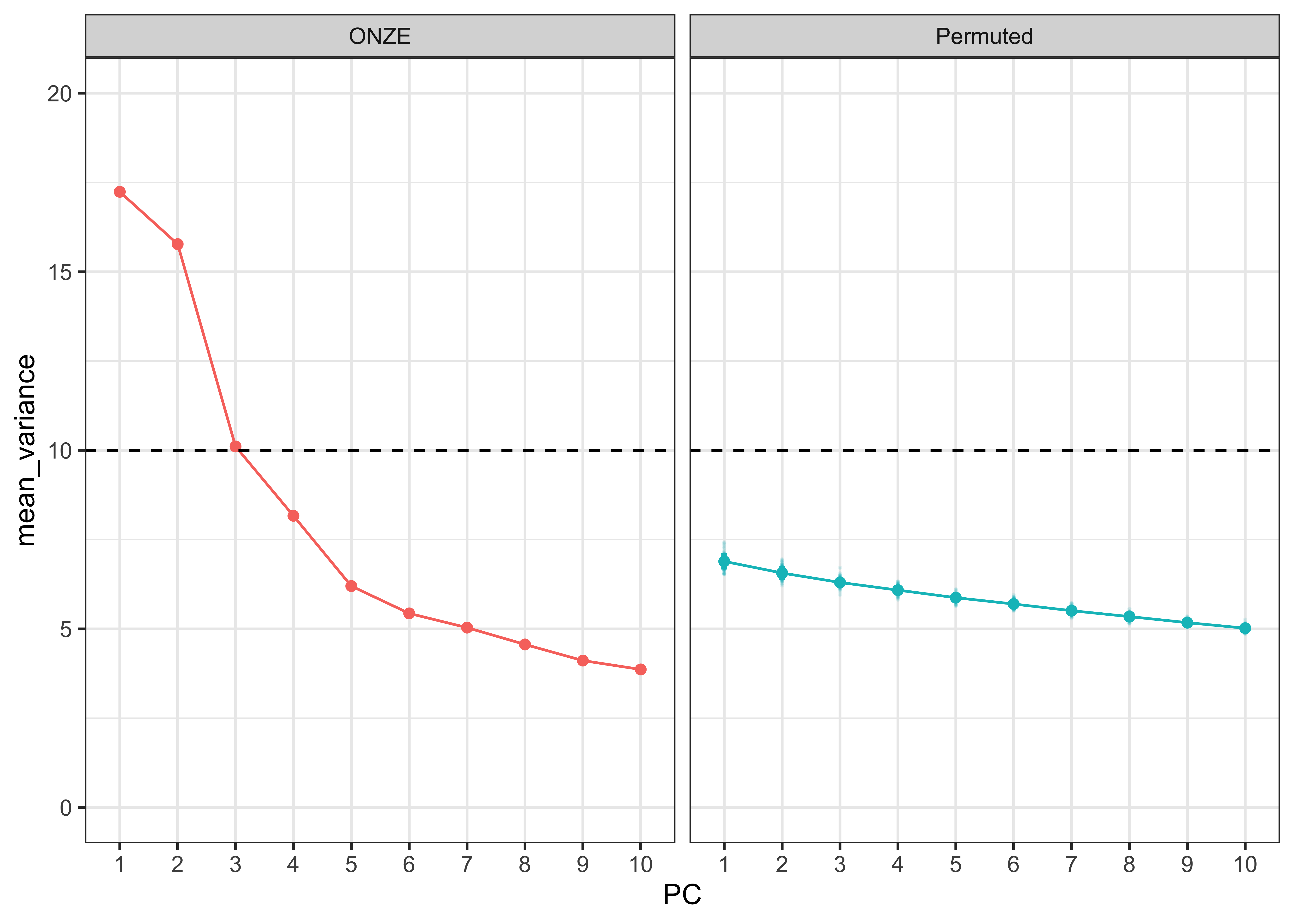

ggsave(plot = PCA_variance_permuted_plot, filename = "Figures/PCA_scree.png", width = 7, height = 5, dpi = 300)

#store these in a data frame for ease of plotting
PC1_loadings <- PC1_loadings %>%
  as.data.frame() %>%#convert to a data frame
  dplyr::rename(Loading = 1) %>% #rename the variable
  mutate(variable = row.names(.), #add variable to identify which intercepts are representing each row
         highlight = ifelse(Loading > 0.225 | Loading < -0.225 , "black", "gray"), #for plotting reasons, we want to highlight the variables that contribute the most to the PC, so if the loading is > |0.2| it will plotted in black, if not it will be gray)
         PC1_loadings_abs = abs(Loading), #make the loadings absolute so they are comparable when plotting
         direction = ifelse(Loading < 0, "red", "black"), #define which direction the loading sign was, i.e. red if negative, black if positive
         PC = "PC1",
         Vowel = substr(variable, 4, 10)) %>% #add variable to identify which PC the data is from
  arrange(PC1_loadings_abs) #order the variables based on absolute loading value

#repeat this process for PC2
PC2_loadings <- PC2_loadings %>%
  as.data.frame() %>%
  dplyr::rename(Loading = 1) %>%
  mutate(variable = row.names(.),
         highlight = ifelse(Loading > 0.225 | Loading < -0.225 , "black", "gray"),
         PC2_loadings_abs = abs(Loading),
         direction = ifelse(Loading < 0, "red", "black"),
         PC = "PC2",
         Vowel = substr(variable, 4, 10)) %>%
  arrange(PC2_loadings_abs)

#repeat this process for PC3
PC3_loadings <- PC3_loadings %>%
  as.data.frame() %>%
  dplyr::rename(Loading = 1) %>%
  mutate(variable = row.names(.),
         highlight = ifelse(Loading > 0.225 | Loading < -0.225 , "black", "gray"),
         PC3_loadings_abs = abs(Loading),
         direction = ifelse(Loading < 0, "red", "black"),
         PC = "PC3",
         Vowel = substr(variable, 4, 10)) %>%
  arrange(PC3_loadings_abs)

PCs by Contribution

To visualise how the different variables contribute to the formation of the PC, we can look at their contribution values. These are simply the variable loading squared and then multiplied by 100, giving a value that is interpretable by means of a percent.

The red dashed line in these plots divides the variables on the basis of cumulative variance explained, whereby those variables to the right of the line collectively account for > 50% of the total variance. Thus, our (least arbitrary) way to define a cut-off point for ‘importance’ of the variables is to focus on those contributing > 50%.

The colour and sign of the dots in these plots is defined by the direction of the loadings in the PCA, i.e. - = negative and + = positive.

First we will wrangle the data from the PCA.

PC_loadings_contrib <- intercepts.pca$loadings[,1:3] %>% #get the loadings for PC1, PC2 and PC3
  as.data.frame() %>%
  cbind(get_pca(intercepts.pca, "var")$contrib[,1:3]) %>% #get the contributions
  dplyr::rename(Loading.PC1 = Comp.1,
         Loading.PC2 = Comp.2,
         Loading.PC3 = Comp.3,
         Contribution.PC1 = Dim.1,
         Contribution.PC2 = Dim.2,
         Contribution.PC3 = Dim.3) %>%
  mutate(Variable = row.names(.),
         Vowel = substr(Variable, 4, nchar(Variable))) %>%
  dplyr::select(Variable, Vowel, Loading.PC1:Contribution.PC3) %>%
  pivot_longer(Loading.PC1:Loading.PC3, names_to = "PC", values_to = "Loading") %>%
  arrange(Vowel, Variable, PC) %>%
  mutate(direction = ifelse(Loading < 0, "red", "black")) #define direction of the loadings

PC1

PC1_contrib <- PC_loadings_contrib %>%
  select(-Contribution.PC2, -Contribution.PC3) %>%
  filter(PC == "Loading.PC1") %>%
  arrange(Contribution.PC1) %>%
  mutate(Loading_abs = abs(Loading),
         cumsum_PC1 = round(cumsum(Contribution.PC1), 4),
         highlight = ifelse(cumsum_PC1 < 50, "grey", "black"),
         highlight1 = ifelse(cumsum_PC1 < 50, 0.5, 1),
         direction1 = direction,
         direction_lab = ifelse(direction1=="red","–", "+"))
  
PC1_contrib_plot <- ggplot(PC1_contrib, aes(x=reorder(Variable, Contribution.PC1), y=Contribution.PC1)) + #have the variable name on the x axis and loading value on the y
  geom_text(aes(alpha = highlight, label=ifelse(PC1_contrib$direction=="red","–", "+")), colour = PC1_contrib$direction, size = 6, fontface="bold", show.legend = FALSE) + 
  xlab("") + #remove the x axis title
  ylab("PC1 contribution (%)") +
  geom_vline(xintercept = 16.5, color = "red", linetype = "dashed") + #add a red dashed line to identify the 0.2 cut off
  scale_alpha_manual(values=c(1, 0.3)) +
  theme_bw() + #set the aesthetics of the plot
  theme(axis.text.x = element_text(angle = 90, hjust = 1, colour = PC1_contrib$highlight, size = 14, face = "bold"),
        axis.text.y = element_text(size = 14, face = "bold"),
        axis.title = element_text(size = 14, face = "bold")) #modify the x axis variable names so they are rotated and highlighted

PC1_contrib_plot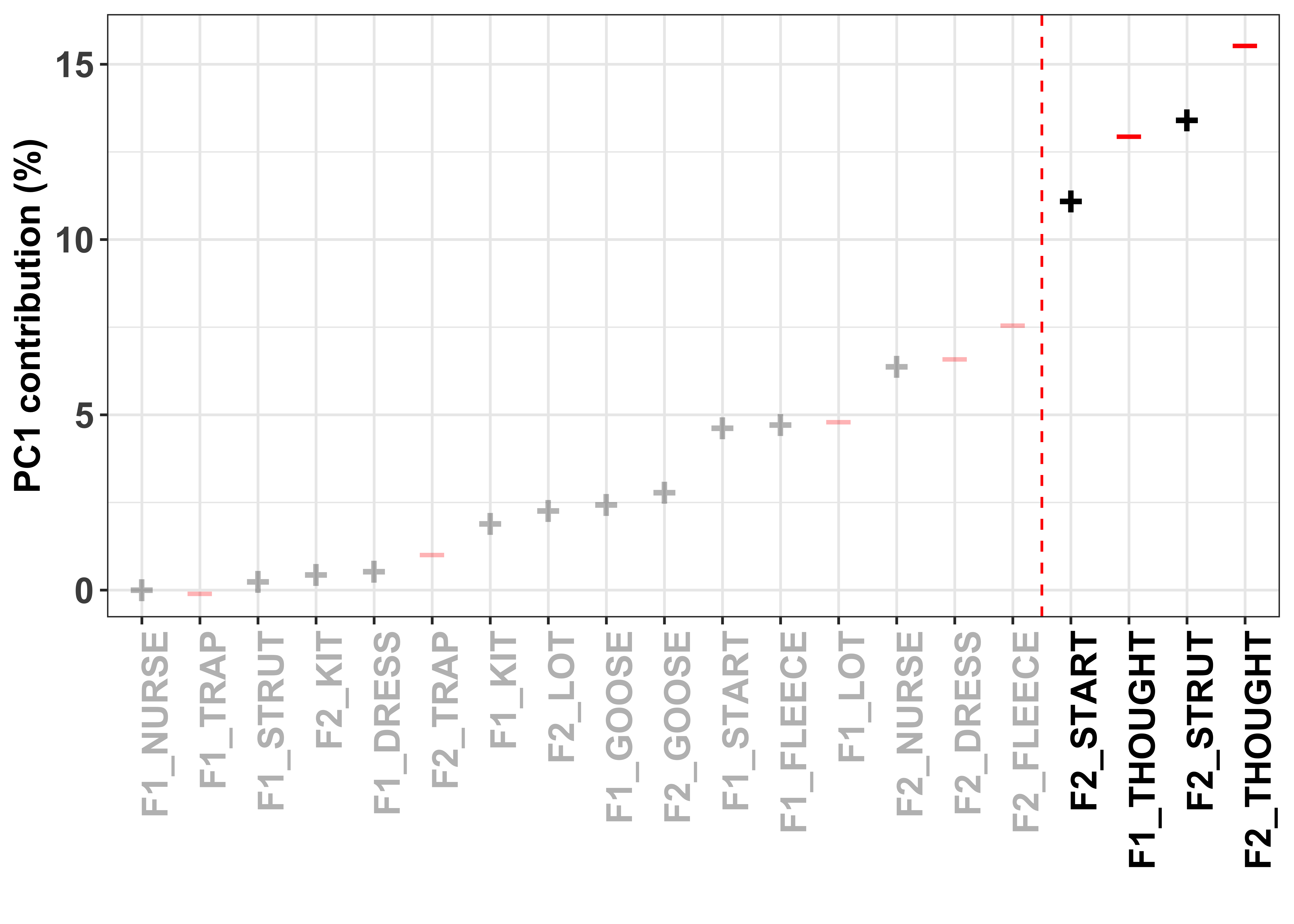

# ggsave(plot = PC1_contrib_plot, filename = "Figures/PC1_contrib_plot.png", width = 8, height = 5, dpi = 300)

PC2

PC2_contrib <- PC_loadings_contrib %>%
  select(-Contribution.PC1, -Contribution.PC3) %>%
  filter(PC == "Loading.PC2") %>%
  arrange(Contribution.PC2) %>%
  mutate(Loading_abs = abs(Loading),
         cumsum_PC2 = round(cumsum(Contribution.PC2), 4),
         highlight = ifelse(cumsum_PC2 < 50, "grey", "black"),
         highlight1 = ifelse(cumsum_PC2 < 50, 0.5, 1),
         direction1 = direction,
         direction_lab = ifelse(direction1=="red","–", "+"))
  
PC2_contrib_plot <- ggplot(PC2_contrib, aes(x=reorder(Variable, Contribution.PC2), y=Contribution.PC2)) + #have the variable name on the x axis and loading value on the y
  geom_text(aes(alpha = highlight, label=ifelse(PC2_contrib$direction=="red","–", "+")), colour = PC2_contrib$direction, size = 6, fontface="bold", show.legend = FALSE) + #add the dots to the plot, with the colour
  xlab("") + #remove the x axis title
  ylab("PC2 contribution (%)") +
  geom_vline(xintercept = 14.5, color = "red", linetype = "dashed") + #add a red dashed line to identify the 0.2 cut off
  scale_alpha_manual(values=c(1, 0.3)) +
  theme_bw() + #set the aesthetics of the plot
  theme(axis.text.x = element_text(angle = 90, hjust = 1, colour = PC2_contrib$highlight, size = 14, face = "bold"),
        axis.text.y = element_text(size = 14, face = "bold"),
        axis.title = element_text(size = 14, face = "bold")) #modify the x axis variable names so they are rotated and highlighted

PC2_contrib_plot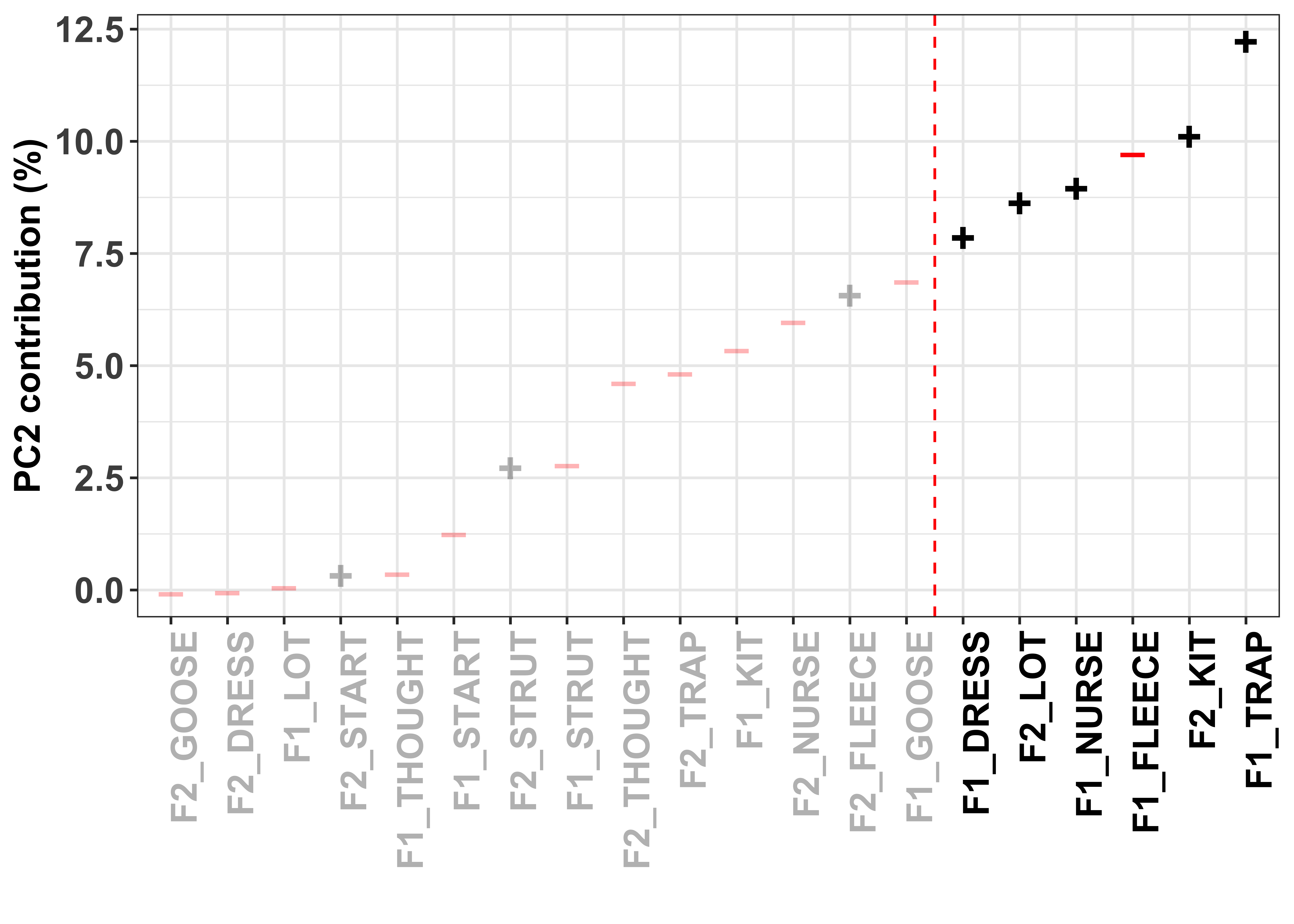

# ggsave(plot = PC2_contrib_plot, filename = "Figures/PC2_contrib_plot.png", width = 8, height = 5, dpi = 300)

PC3

PC3_contrib <- PC_loadings_contrib %>%
  select(-Contribution.PC1, -Contribution.PC2) %>%
  filter(PC == "Loading.PC3") %>%
  arrange(Contribution.PC3) %>%
  mutate(Loading_abs = abs(Loading),
         cumsum_PC3 = round(cumsum(Contribution.PC3), 4),
         highlight = ifelse(cumsum_PC3 < 50, "grey", "black"),
         highlight1 = ifelse(cumsum_PC3 < 50, 0.5, 1),
         direction1 = direction,
         direction_lab = ifelse(direction1=="red","–", "+"))
  
PC3_contrib_plot <- ggplot(PC3_contrib, aes(x=reorder(Variable, Contribution.PC3), y=Contribution.PC3)) + #have the variable name on the x axis and loading value on the y
  geom_text(aes(alpha = highlight, label=ifelse(PC3_contrib$direction=="red","–", "+")), colour = PC3_contrib$direction, size = 6, fontface="bold", show.legend = FALSE) + 
  xlab("") + #remove the x axis title
  ylab("PC3 contribution (%)") +
  geom_vline(xintercept = 16.5, color = "red", linetype = "dashed") + #add a red dashed line to identify the 0.2 cut off
  scale_alpha_manual(values=c(1, 0.3)) +
  theme_bw() + #set the aesthetics of the plot
  theme(axis.text.x = element_text(angle = 90, hjust = 1, colour = PC3_contrib$highlight, size = 14, face = "bold"),
        axis.text.y = element_text(size = 14, face = "bold"),
        axis.title = element_text(size = 14, face = "bold")) #modify the x axis variable names so they are rotated and highlighted

PC3_contrib_plot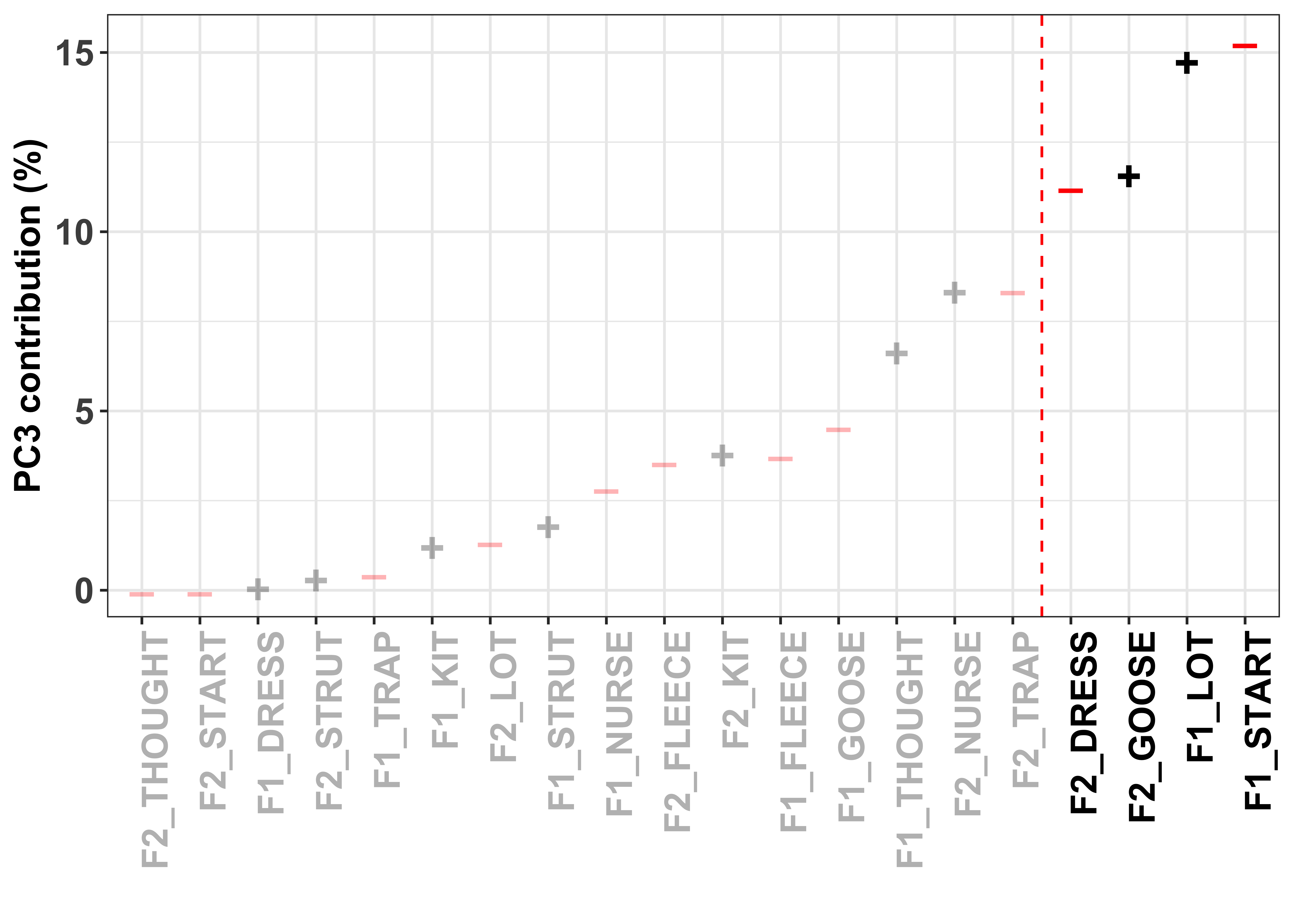

# ggsave(plot = PC3_contrib_plot, filename = "Figures/PC3_contrib_plot.png", width = 8, height = 5, dpi = 300)

Visualisation in vowel space

In order to understand how these variables are co-varying together, we can re-interpret the dot plots in terms of F1/F2 vowel space. This will allow us to explore our theoretically motivated interpretation that these PCs represent changes in F1/F2 over time, thus demonstrating that the PCs may be representing ‘leaders’ and ‘laggers’ of sound change.

1. We will plot how the vowel space in New Zealand English has changed over the course of the dataset (defined by year of birth), based on the GAMM modelling performed in earlier models.

2. We then visualise how the vowel spaces of the speakers in PC1, PC2 and PC3 also change (defined by the PCA scores), this interpretation will be driven by the weighting of the variable loadings on each PC (as shown in the dot plots). This will done in 3 different ways:

• GAM smooths

• Vowel plots

• Animations

In order to generate these plots, we have to run more GAMMs predicting either F1 or F2 (normalised), by the PCA scores, this will provide us with predicted model values, that show the trajectories based on the PCA scores (i.e. going from negative to positive values).

Note, the direction of the PCA scores (for PC1, PC2 and PC3) have been reversed in the figures, i.e. negative scores are switched to positive and vice versa. This is purely for visualisation purposes as it helps the interpretation in terms of change over time. This does not affect any underlying importance of the actual scores, the direction (+/-) is arbitrary in PCA and remains the same as long as all values are switched, which they have been.

Sound change

Visualisation by GAM smooth

Plotting change in normalised (Lobanov 2.0) F1 (red lines) and F2 (blue lines)

• x axis = year of birth

• y axis = normalised F1/F2

• smoothed lines = GAM fit

year of birth

Load in the models and get the predicted values.

These steps are pre-run (they are big objects in R), but the resulting data can be found in the Data > Models folder, saved as mod_pred_yob_values.rds and mod_pred_yobgender_values.rds

mod_pred_yob_values <-  readRDS("Data/Models/mod_pred_yob_values.rds")

#make a long version of the intercepts
gam_intercepts.tmp_long <- gam_intercepts.tmp %>%
  pivot_longer(F1_DRESS:F2_TRAP, names_to = "Vowel_formant", values_to = "Intercept") %>%
  mutate(Formant = substr(Vowel_formant, 1, 2),
         Vowel = substr(Vowel_formant, 4, max(nchar(Vowel_formant)))) %>%
  left_join(vowels_all %>%
  select(Speaker, participant_year_of_birth, Gender) %>% distinct()) %>%
  left_join(mod_pred_yob_values %>% select(participant_year_of_birth, Vowel, Formant, fit, ll, ul))

#plot the gam smooths predicting F1/F2 per vowel and add the speaker intercepts values
sound_change_plot_smooth <- mod_pred_yob_values %>%
  mutate(Formant = factor(Formant, levels = c("F2", "F1"))) %>%
  ggplot(aes(x = participant_year_of_birth, y = fit, colour = Formant, fill = Formant)) +
  geom_point(data = gam_intercepts.tmp_long %>% mutate(Formant = factor(Formant, levels = c("F2", "F1"))), aes(x = participant_year_of_birth, y = fit + Intercept), size = 0.25, alpha = 0.1) +
  geom_line(size = 1) +
  geom_ribbon(aes(ymin = ll, ymax = ul), alpha = 0.2, colour = NA) +
  scale_x_continuous(breaks = c(1900, 1950)) +
  xlab("Year of birth") +
  ylab("Predicted model fit (Lobanov 2.0)") +
  facet_grid(Formant~Vowel) +
  theme_bw() +
  theme(legend.position = "none", axis.text = element_text(size = 12), axis.title = element_text(size = 14, face = "bold"), strip.text = element_text(size = 12, face = "bold"))

sound_change_plot_smooth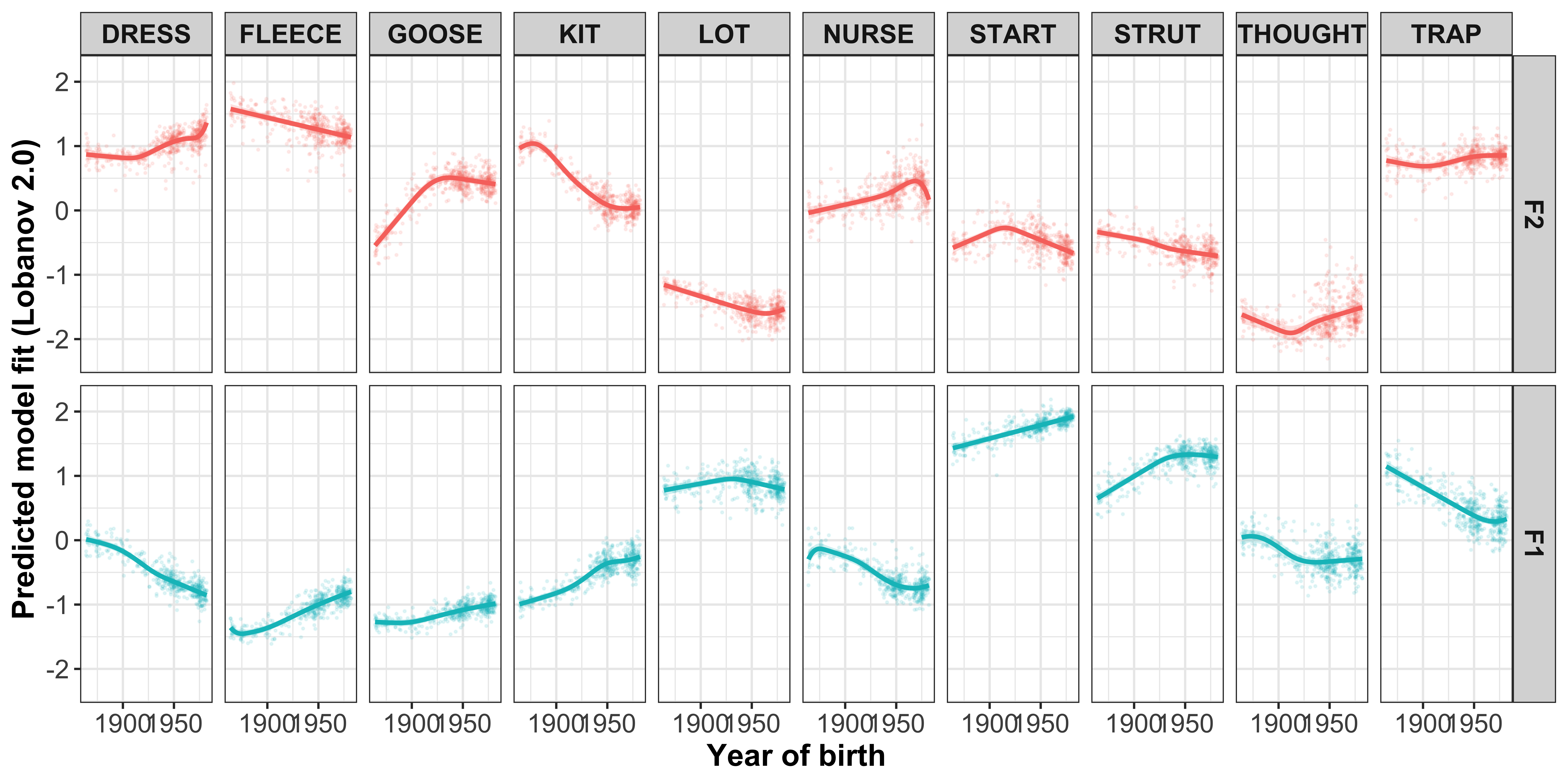

ggsave(plot = sound_change_plot_smooth, filename = "Figures/sound_change_gam.png", width = 12, height = 5, dpi = 600)

year of birth and gender

mod_pred_yobgender_values <- readRDS("Data/Models/mod_pred_yobgender_values.rds")

#plot the gam smooths predicting F1/F2 per vowel and add the per speaker mean values with F or M as the text
sound_change_plot_smooth_gender <- mod_pred_yobgender_values %>%
  mutate(Formant = factor(Formant, levels = c("F2", "F1"))) %>%
  ggplot(aes(x = participant_year_of_birth, y = fit, colour = Formant, linetype = Gender, label = Gender, fill = Formant)) +
  geom_text(data = gam_intercepts.tmp_long %>%
  mutate(Formant = factor(Formant, levels = c("F2", "F1"))), aes(x = participant_year_of_birth, y = fit + Intercept), size = 1, alpha = 0.5) +
  geom_line(size = 1) +
  geom_ribbon(aes(ymin = ll, ymax = ul), alpha = 0.2, colour = NA) +
  scale_x_continuous(breaks = c(1900, 1950)) +
  xlab("Year of birth") +
  ylab("Predicted model fit (Lobanov 2.0)") +
  facet_grid(Formant~Vowel) +
  theme_bw() +
  theme(legend.position = "top", axis.text = element_text(size = 12), axis.title = element_text(size = 14, face = "bold"), strip.text = element_text(size = 12, face = "bold")) +
  guides(linetype=guide_legend(override.aes=list(fill=NA)))

sound_change_plot_smooth_gender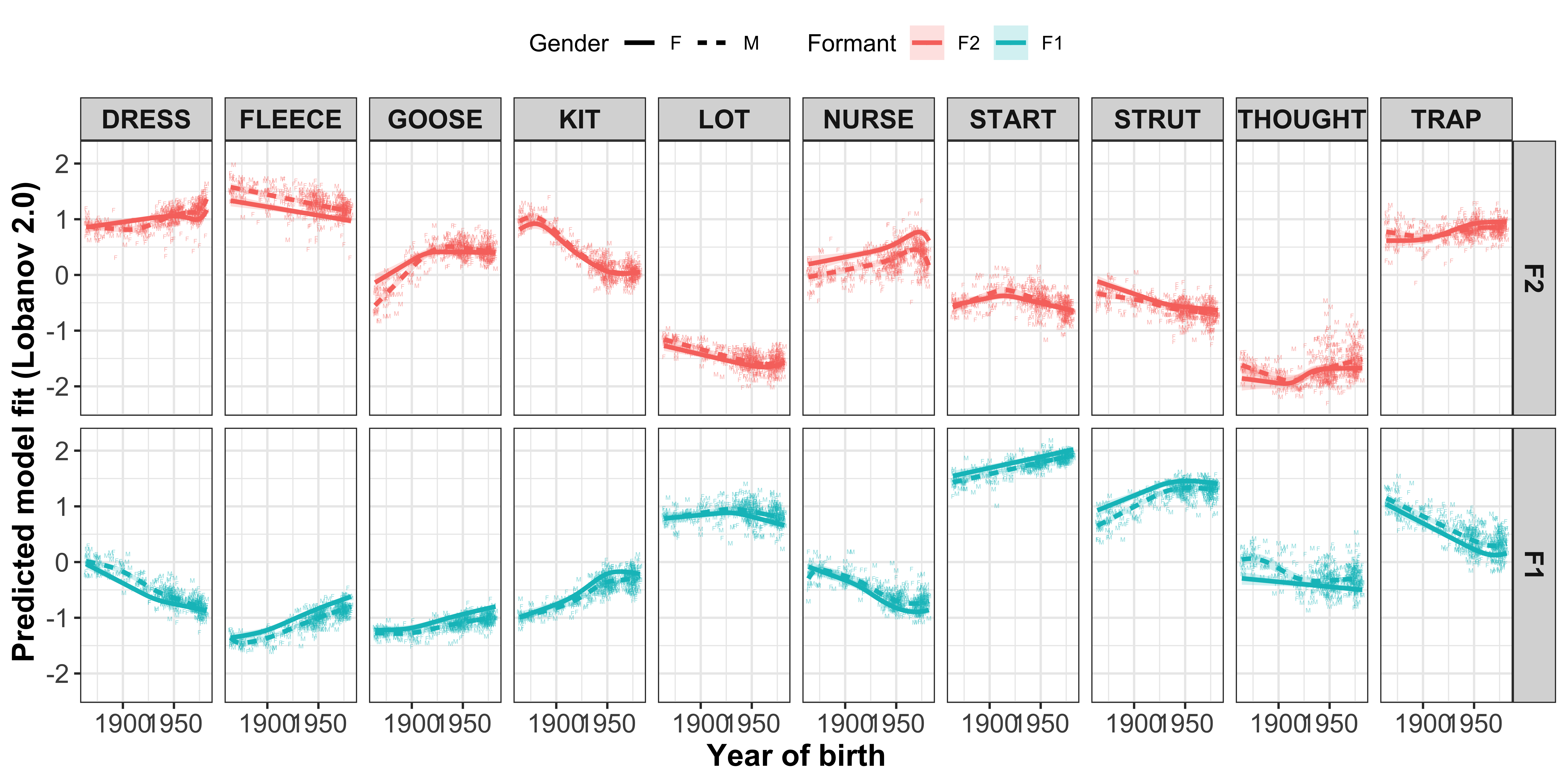

ggsave(plot = sound_change_plot_smooth_gender, filename = "Figures/sound_change_gam_gender.png", width = 10, height = 5, dpi = 600)

Visualisation in F1/F2 space

We can convert the data from the above plot in (Lobanov 2.0 normalised) F1/F2 space, to see the changes in a more conventional vowel space plot

• x axis = F2

• y axis = F1

• colours = lexical set of vowel

• lines = trajectory of the F1/F2 in terms of year of birth (1857 - 1988)

• vowel labels = start point of the vowel trajectory (oldest year of birth: 1857)

• arrows = end point of the trajectory (youngest year of birth: 1988)

#transform data so there are separate columns for F1 and F2
sound_change_plot_data <- mod_pred_yob_values %>%
  select(participant_year_of_birth, fit, Vowel, Formant) %>%
  pivot_wider(names_from = Formant, values_from = fit) #transform the data to wide format so there are separate F1 and F2 variables

#make data frame to plot starting point, this will give the vowel labels based on the smallest year of birth coordinates
sound_change_labels1 <- sound_change_plot_data %>%
  group_by(Vowel) %>%
  filter(participant_year_of_birth == min(participant_year_of_birth))

#make data frame to plot end point, this will give the arrow at the end of the paths based on the largest year of birth coordinates
sound_change_labels2 <- sound_change_plot_data %>%
  group_by(Vowel) %>%
  top_n(wt = participant_year_of_birth, n = 2)

#plot
sound_change_plot <- sound_change_plot_data %>%
  #set general aesthetics
  ggplot(aes(x = F2, y = F1, colour = Vowel, alpha = participant_year_of_birth, group = Vowel)) +
  #add year of birth change trajectories
  geom_path(size = 0.5, show.legend = FALSE) +
  #add end points (this gives the arrows)
  geom_path(data = sound_change_labels2, aes(x = F2, y = F1, colour = Vowel, group = Vowel),
            arrow = arrow(ends = "last", type = "closed", length = unit(0.2, "cm")),
            inherit.aes = FALSE, show.legend = FALSE) +
  #plot the vowel labels
  geom_text(data = sound_change_labels1, aes(x = F2, y = F1, colour = Vowel, group = Vowel, label = Vowel), inherit.aes = FALSE, show.legend = FALSE) +
  #label the axes
  xlab("F2 (normalised)") +
  ylab("F1 (normalised)") +
  #scale the size so the path is not too wide
  scale_size_continuous(range = c(0.2,1)) +
  #reverse the axes to follow conventional vowel plotting
  scale_x_reverse(limits = c(2,-2), position = "top") +
  scale_y_reverse(limits = c(2.3,-2), position = "right") +
  #set the colours
  scale_color_manual(values = c("#9590FF", "#D89000", "#A3A500", "#39B600", "#00BF7D",
                                 "#00BFC4", "#00B0F6", "#F8766D", "#E76BF3", "#FF62BC")) +
  #add a title
  # labs(title = "A) Change over time\n     ") +
  #set the theme
  theme_bw() +
  #make title bold
  theme(plot.title = element_text(face="bold"))

sound_change_plot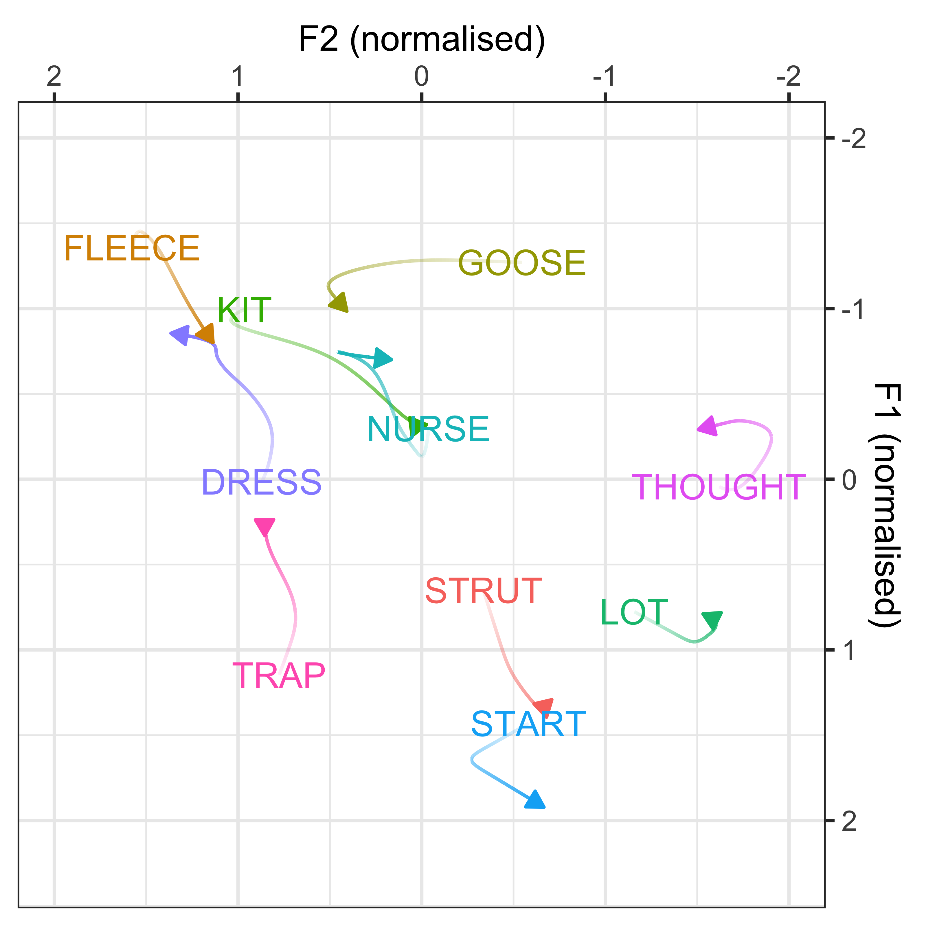

ggsave(plot = sound_change_plot, filename = "Figures/sound_change_static.png", width = 5.5, height = 5.5, dpi = 300)

Visualisation by animation

We can also recreate the above plot in 3 dimensional space, where the trajectories are animated.

• x axis = F2

• y axis = F1

• colours = lexical set of vowel

• movement = trajectory of the F1/F2 in terms of year of birth (1857 - 1988)

• trails = the previous positions of the vowels

sound_change_plot_animation <- sound_change_plot_data %>%
  #set general aesthetics
  ggplot(aes(x = F2, y = F1, colour = Vowel, group = Vowel, label = Vowel)) +
  geom_text(aes(fontface = 2), size = 5, show.legend = FALSE) +
  # geom_point() +
  geom_path() +
  #label the axes
  xlab("F2 (normalised)") +
  ylab("F1 (normalised)") +
  #reverse the axes to follow conventional vowel plotting
  scale_x_reverse(limits = c(2,-2), position = "top") +
  scale_y_reverse(limits = c(2.3,-2), position = "right") +
  #set the colours
  scale_color_manual(values = c("#9590FF", "#D89000", "#A3A500", "#39B600", "#00BF7D",
                                 "#00BFC4", "#00B0F6", "#F8766D", "#E76BF3", "#FF62BC")) +
  #add a title
  labs(caption = 'Year of birth: {round(frame_along, 0)}') +
  #set the theme
  theme_bw() +
  #make text more visible
  theme(axis.title = element_text(size = 14, face = "bold"),
        axis.text.x = element_text(size = 14, face = "bold"),
        axis.text.y = element_text(size = 14, face = "bold", angle = 270),
        axis.ticks = element_blank(),
        plot.caption = element_text(size = 30, hjust = 0),
        legend.position = "none") +
  #set the variable for the animation transition i.e. the time dimension
  transition_reveal(participant_year_of_birth) +
  #add in a trail to see the path
  # shadow_trail(max_frames = 100, alpha = 0.1) +
  ease_aes('linear')

sound_change_plot_animation <- animate(sound_change_plot_animation, nframes = 200, fps = 5, rewind = FALSE, start_pause = 10, end_pause = 10, duration = 20)

# animate(sound_change_plot_animation, nframes = 200, fps = 5, rewind = FALSE, start_pause = 10, end_pause = 10, duration = 20, height = 800, width =800)

anim_save(sound_change_plot_animation, filename = "Figures/sound_change_animation.gif")

sound_change_plot_animation

PC scores

To understand how the PCs vary in terms of the co-variation between the vowel-formants, we want to inspect the PC scores. Within each of the PCs, there will be speakers who typify the co-variation seen in the dot plots. This is shown through the PC scores, with each speaker assigned a different score for each of the PCs. These scores can be interpreted in a similar way to the loadings - the larger your score (either +/-), the more that speaker contributes to the co-variation.

We can explore the PC scores to:

• Assess the relationship between the scores and the intercepts

• Visualise the vowel spaces of speakers with +/- scores

• Understand how these speakers differ in terms of F1~F2 space for the vowel-formants contributing most to each PC

• Inspect the relationship between the PC scores and directions of sound change

• Test if the PC scores are independent of the socio-demographic variables included in the sound change GAMMs

Each speaker has a PC score within each of the PCs (which can be found in intercepts.pca$scores), thus we need to extract this information and combine it with the speaker’s social information (which can be found in vowels_all).

Relationship between intercepts and PC scores

First let’s visualise the relationship between the PC scores and the speaker intercepts. This will show us if speakers with +/- scores have +/- intercepts. Our prediction is that those with the largest PC scores will have large intercepts. When we are referring to ‘large’ here, we are talking about absolute values, where + and - values are important.

The vowel-formants that contribute most to a PC (highlighted by the yellow boxes in the plot below) are those we are most interested in and should show a clear slope in the regression fits.

#extract the PCA scores for the first 3 PCs from the PCA
PC_speaker_loadings <- as.data.frame(intercepts.pca$scores[,1:3]) %>% #the loadings are stored in the scores part of the intercepts.pca object
  mutate(Speaker = gam_intercepts.tmp$Speaker) #create a Speaker variable with the speaker names

#get speaker's social information and combine it with the speaker intercepts and then the PC loadings
PC_speaker_loadings <-  vowels_all %>%
  dplyr::select(Speaker, Corpus, Gender, participant_year_of_birth) %>% #choose the variables of interest from vowels_all
  distinct() %>% #make one row for each speaker
  left_join(., gam_intercepts.tmp, by = "Speaker") %>% #combine the social information with the intercepts
  left_join(., PC_speaker_loadings, by = "Speaker") #combine this with the PC loadings

#add the PCA scores from PC1, PC2 and PC3
vowels_all <- vowels_all %>%
  left_join(PC_speaker_loadings[, c("Speaker", "Comp.1", "Comp.2", "Comp.3")])

PC_variable_loadings <- data.frame(intercepts.pca$loadings[,1:3]) %>%
  mutate(name = row.names(.),
         Formant = substr(name, 1, 2), #add extra variables
         Vowel = substr(name, 4, max(nchar(name)))) %>%
  rename(PC1_loading = 1,
         PC2_loading = 2,
         PC3_loading = 3)

#extract the PCA scores for the first 3 PCs from the PCA
PC_speaker_loadings1 <- as.data.frame(intercepts.pca$scores[,1:3]) %>% #the loadings are stored in the scores part of the intercepts.pca object
  mutate(Speaker = gam_intercepts.tmp$Speaker) %>%
  left_join(vowels_all %>% select(Speaker, participant_year_of_birth, Gender) %>% distinct())

PC = c(1:3)

gam_intercepts.tmp_long1 <- intercepts.pca$scores[,PC] %*% t(intercepts.pca$loadings[,PC]) %>%
  data.frame() %>%
  mutate(Speaker = gam_intercepts.tmp$Speaker) %>% #add speaker names
  select(Speaker, 1:ncol(.)-1) %>% #reorder the variables
  pivot_longer(F1_DRESS:F2_TRAP) %>% #make data long
  left_join(gam_intercepts.tmp %>% pivot_longer(F1_DRESS:F2_TRAP, values_to = "intercepts")) %>% #add the original intercepts
  mutate(Formant = substr(name, 1, 2), #add extra variables
         Vowel = substr(name, 4, max(nchar(name))),
         mod = paste0(Formant, "_intercepts")) %>%
  left_join(PC_speaker_loadings %>% select(Speaker:participant_year_of_birth, Gender, Comp.1, Comp.2, Comp.3)) %>%
  left_join(mod_pred_yob_values %>% select(participant_year_of_birth, fit, ll, ul, Vowel, Formant)) %>%
  left_join(PC_variable_loadings) %>%
  left_join(PC_variable_loadings %>% group_by(Vowel) %>% summarise(PC1_loading_max = max(abs(PC1_loading)), PC2_loading_max = max(abs(PC2_loading)), PC3_loading_max = max(abs(PC3_loading)))) %>%
  mutate(intercepts1 = intercepts + fit,
         Formant = factor(Formant, levels = c("F2", "F1"), ordered = TRUE))

gam_intercepts.tmp_long1_test <- gam_intercepts.tmp_long1 %>%
  pivot_longer(Comp.1:Comp.3, names_to = "Comp", values_to = "Comp_score") %>%
  left_join(., rbind(PC1_contrib %>% ungroup() %>% select(Variable, PC, highlight),
      PC2_contrib %>% ungroup() %>% select(Variable, PC, highlight),
      PC3_contrib %>% ungroup() %>% select(Variable, PC, highlight)) %>%
        rename(name = Variable,
               Comp = PC) %>%
        mutate(Comp = gsub(x = Comp, "Loading.PC", "Comp.")))

ggplot(data = gam_intercepts.tmp_long1_test, aes(x = -Comp_score, y = intercepts, colour = Comp)) +
  geom_point(size = 0.5, alpha = 0.1, colour = "black") +
  # geom_point(aes(x = Comp_score, y = intercepts1), colour = "red", size = 0.2, alpha = 0.1) +
  geom_smooth(method = "lm") +
  # geom_smooth(aes(x = intercepts, y = intercepts1), colour = "red", method = "lm") +
  geom_abline(slope = 0, linetype = 2) +
  geom_rect(data = gam_intercepts.tmp_long1_test %>% filter(highlight == "black"), aes(xmin = -7, xmax = 7, ymin = -1.2, ymax = 1.2), alpha = 0, colour = "yellow") +
  # scale_colour_viridis_c() +
  xlab("PC score") +
  facet_grid(Comp+Formant~Vowel) +
  theme_bw() +
  theme(legend.position = "none")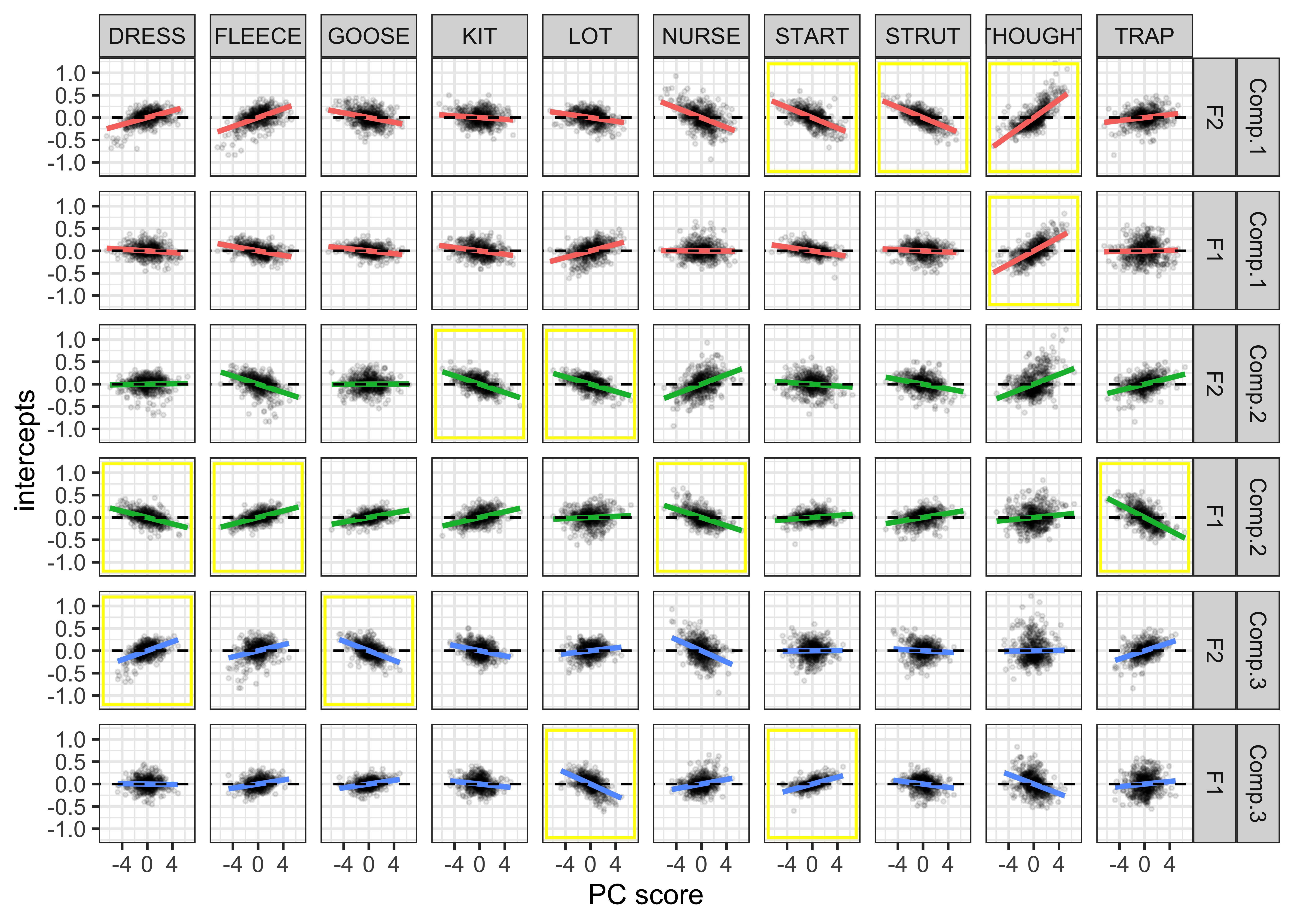

Regression models for intercepts ~ PC score

As the above plot is just a visualisation, we want to now run the regressions.

For each PC, we will run a regression for each vowel-formant, where we predict the speaker intercept by the speaker PC scores. We are not necessarily interested in the p values of these models as they are mainly for visualisation of the relationship.

mod_pred_PC1_values <- data.frame(intercepts = numeric(),
                                  Comp.1 = numeric(),
                                  residuals = numeric(),
                                  fitted.values = numeric(),
                                  residuals1 = numeric(),
                                  fitted.values1 = numeric(),
                                  mod = character())

for (i in levels(factor(gam_intercepts.tmp_long1$name))) {
  lm1 <- lm(intercepts ~ Comp.1, data = gam_intercepts.tmp_long1, subset = name == i)
  lm1_values <- cbind(lm1[["model"]], lm1[["residuals"]], lm1[["fitted.values"]]) %>%
    rename(residuals = 3, fitted.values = 4) %>%
    mutate(diff = residuals + fitted.values,
           mod = i,
           Formant = substr(i, 1, 2),
           Vowel = substr(i, 4, nchar(i)))

  lm2 <- lm(intercepts1 ~ Comp.1, data = gam_intercepts.tmp_long1, subset = name == i)
  lm2_values <- cbind(lm2[["model"]], lm2[["residuals"]], lm2[["fitted.values"]]) %>%
    rename(residuals1 = 3, fitted.values1 = 4) %>%
    mutate(diff1 = residuals1 + fitted.values1)

  lm1_values <- lm1_values %>%
    left_join(lm2_values)

  mod_pred_PC1_values <<- rbind(mod_pred_PC1_values, lm1_values)
}

mod_pred_PC1_values_plot <- mod_pred_PC1_values %>%
  select(Vowel, Formant, Comp.1, intercepts, fitted.values, intercepts1, fitted.values1) %>%
  pivot_wider(names_from = Formant, values_from = c(intercepts, fitted.values, intercepts1, fitted.values1)) %>%
  group_by(Vowel) %>%
  mutate(id = 1:481) %>%
  left_join(gam_intercepts.tmp_long1 %>%
              select(Speaker, Vowel, Formant, PC1_loading, PC1_loading_max, fit, intercepts, intercepts1, participant_year_of_birth) %>%
              pivot_wider(names_from = Formant, values_from = c(fit, intercepts, intercepts1, PC1_loading)) %>%
              distinct())

mod_pred_PC2_values <- data.frame(intercepts = numeric(),
                                  Comp.2 = numeric(),
                                  residuals = numeric(),
                                  fitted.values = numeric(),
                                  residuals1 = numeric(),
                                  fitted.values1 = numeric(),
                                  mod = character())

for (i in levels(factor(gam_intercepts.tmp_long1$name))) {
  lm1 <- lm(intercepts ~ Comp.2, data = gam_intercepts.tmp_long1, subset = name == i)
  lm1_values <- cbind(lm1[["model"]], lm1[["residuals"]], lm1[["fitted.values"]]) %>%
    rename(residuals = 3, fitted.values = 4) %>%
    mutate(diff = residuals + fitted.values,
           mod = i,
           Formant = substr(i, 1, 2),
           Vowel = substr(i, 4, nchar(i)))

  lm2 <- lm(intercepts1 ~ Comp.2, data = gam_intercepts.tmp_long1, subset = name == i)
  lm2_values <- cbind(lm2[["model"]], lm2[["residuals"]], lm2[["fitted.values"]]) %>%
    rename(residuals1 = 3, fitted.values1 = 4) %>%
    mutate(diff1 = residuals1 + fitted.values1)

  lm1_values <- lm1_values %>%
    left_join(lm2_values)

  mod_pred_PC2_values <<- rbind(mod_pred_PC2_values, lm1_values)
}

mod_pred_PC2_values_plot <- mod_pred_PC2_values %>%
  select(Vowel, Formant, Comp.2, intercepts, fitted.values, intercepts1, fitted.values1) %>%
  pivot_wider(names_from = Formant, values_from = c(intercepts, fitted.values, intercepts1, fitted.values1)) %>%
  group_by(Vowel) %>%
  mutate(id = 1:481) %>%
  left_join(gam_intercepts.tmp_long1 %>%
              select(Speaker, Vowel, Formant, PC2_loading, PC2_loading_max, fit, intercepts, intercepts1, participant_year_of_birth) %>%
              pivot_wider(names_from = Formant, values_from = c(fit, intercepts, intercepts1, PC2_loading)) %>%
              distinct())

mod_pred_PC3_values <- data.frame(intercepts = numeric(),
                                  Comp.3 = numeric(),
                                  residuals = numeric(),
                                  fitted.values = numeric(),
                                  residuals1 = numeric(),
                                  fitted.values1 = numeric(),
                                  mod = character())

for (i in levels(factor(gam_intercepts.tmp_long1$name))) {
  lm1 <- lm(intercepts ~ Comp.3, data = gam_intercepts.tmp_long1, subset = name == i)
  lm1_values <- cbind(lm1[["model"]], lm1[["residuals"]], lm1[["fitted.values"]]) %>%
    rename(residuals = 3, fitted.values = 4) %>%
    mutate(diff = residuals + fitted.values,
           mod = i,
           Formant = substr(i, 1, 2),
           Vowel = substr(i, 4, nchar(i)))

  lm2 <- lm(intercepts1 ~ Comp.3, data = gam_intercepts.tmp_long1, subset = name == i)
  lm2_values <- cbind(lm2[["model"]], lm2[["residuals"]], lm2[["fitted.values"]]) %>%
    rename(residuals1 = 3, fitted.values1 = 4) %>%
    mutate(diff1 = residuals1 + fitted.values1)

  lm1_values <- lm1_values %>%
    left_join(lm2_values)

  mod_pred_PC3_values <<- rbind(mod_pred_PC3_values, lm1_values)
}

mod_pred_PC3_values_plot <- mod_pred_PC3_values %>%
  select(Vowel, Formant, Comp.3, intercepts, fitted.values, intercepts1, fitted.values1) %>%
  pivot_wider(names_from = Formant, values_from = c(intercepts, fitted.values, intercepts1, fitted.values1)) %>%
  group_by(Vowel) %>%
  mutate(id = 1:481) %>%
  left_join(gam_intercepts.tmp_long1 %>%
              select(Speaker, Vowel, Formant, PC3_loading, PC3_loading_max, fit, intercepts, intercepts1, participant_year_of_birth) %>%
              pivot_wider(names_from = Formant, values_from = c(fit, intercepts, intercepts1, PC3_loading)) %>%
              distinct())

mod_pred_PC_values <- cbind(mod_pred_PC1_values_plot %>%
          select(Comp.1, Vowel, fitted.values1_F1, fitted.values1_F2) %>%
          dplyr::rename(F1_PC1 = fitted.values1_F1,
                F2_PC1 = fitted.values1_F2),
          mod_pred_PC2_values_plot %>%
          select(Comp.2, Vowel, fitted.values1_F1, fitted.values1_F2) %>%
          dplyr::rename(F1_PC2 = fitted.values1_F1,
                F2_PC2 = fitted.values1_F2),
          mod_pred_PC3_values_plot %>%
          select(Comp.3, Vowel, fitted.values1_F1, fitted.values1_F2) %>%
          dplyr::rename(F1_PC3 = fitted.values1_F1,
                F2_PC3 = fitted.values1_F2))

Visualisation in F1~F2 space

Now we have the predicted values from the regression models, we can transform that data to visualise it in terms of F1~F2 space.

In the plots below, there is a vowel space plotted for each of the 3 PCs. The plots show:

• The location of the speaker intercepts (calculated by adding them to the GAMM model predictions for year of birth). These are plotted as the points and coloured by the speaker PC score (+ = green, - = black)

• The direction of the regression model predictions. Plotted as the green to black trajectories. The wider and larger the trajectories, the more important the vowel is to the PC

• The vowel label. Plotted as text, the size and yellowness indicates the importance of the vowel to the PC (large and yellow labels account for more variance in the PC). The position is based on the point where the regression trajectory is for the speakers with smallest negative PC score

The plots can be used to interpret the directionality of the vowel-formants in the PC, providing a schematic of where speakers with +/- PC scores are in terms of F1~F2 space.

mod_pred_PC1_values_vowel_plot <- mod_pred_PC1_values_plot %>%
  ggplot(aes(x = fitted.values1_F2, y = fitted.values1_F1, colour = -Comp.1, size = PC1_loading_max, group = Vowel)) +
  geom_point(aes(x = intercepts1_F2, y = intercepts1_F1), size = 0.4, alpha = 0.5) +
  # geom_path(data = mod_pred_PC3_values_plot %>% arrange(Vowel, participant_year_of_birth), aes(x = fit_F2, y = fit_F1, group = Vowel), size = 1, colour = "red") +
  geom_line() +
  geom_label(data = mod_pred_PC1_values_plot %>%
  mutate(fitted.values2_F1 = ifelse(Vowel %in% c("FLEECE", "DRESS", "GOOSE"), 1,
                                    ifelse(Vowel %in% c("THOUGHT", "LOT"), 0, 0.5)),
         fitted.values2_F2 = ifelse(Vowel %in% c("STRUT", "START", "NURSE", "GOOSE"), 1,
                                    ifelse(Vowel %in% c("DRESS", "FLEECE"), 0, 0.5))) %>%
               filter(-Comp.1 == min(-Comp.1)), aes(label = Vowel, fill = rescale(PC1_loading_max^2, to = c(0, 1)), vjust = fitted.values2_F1, hjust = fitted.values2_F2), label.padding = unit(0.1, "lines"), colour = "black", show.legend = FALSE) +
  xlab("F2 (normalised)") +
  ylab("F1 (normalised)") +
  scale_x_reverse(position = "top", limits = c(2.4, -3)) +
  scale_y_reverse(position = "right") +
  scale_colour_gradient2(name = "PC1 score", low = "black", mid = "white" , high = "#7CAE00",
                         midpoint=0, breaks = c(-3, 0, 3)) +
  scale_fill_gradient(low = "white", high = "yellow", guide = "none") +
  scale_size_continuous(range = c(1, 5), guide = "none") +
  # facet_wrap(~Vowel) +
  theme_bw() +
  theme(legend.position = "bottom", axis.title = element_text(size = 14, face = "bold"), legend.title = element_text(size = 14, face = "bold"), legend.text = element_text(size = 14, face = "bold"))

mod_pred_PC1_values_vowel_plot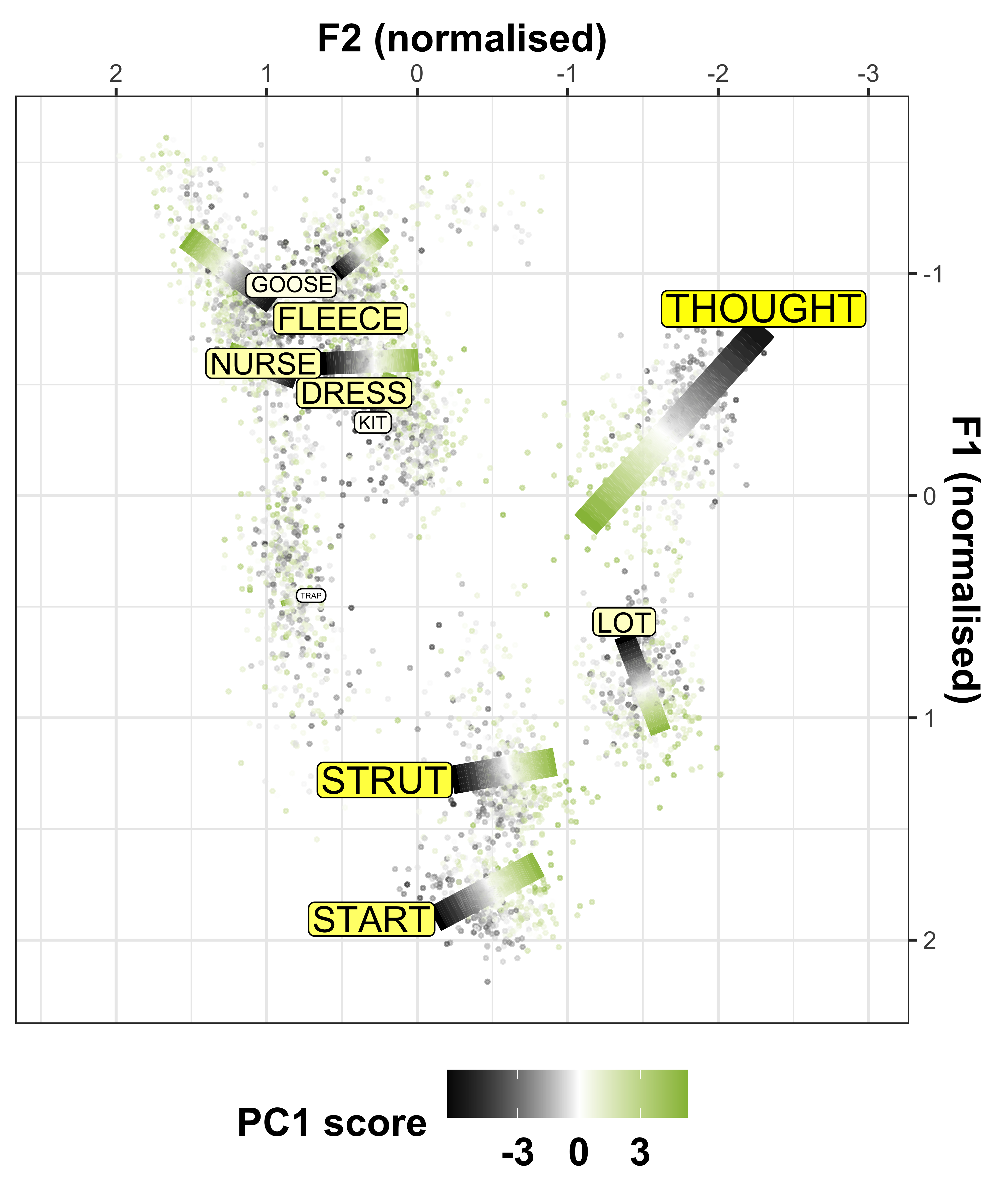

ggsave(plot = mod_pred_PC1_values_vowel_plot, filename = "Figures/mod_pred_PC1_values_vowel_plot.png", width = 7, height = 7, dpi = 400)

mod_pred_PC2_values_vowel_plot <- mod_pred_PC2_values_plot %>%
  ggplot(aes(x = fitted.values1_F2, y = fitted.values1_F1, colour = -Comp.2, size = PC2_loading_max, group = Vowel)) +
  geom_point(aes(x = intercepts1_F2, y = intercepts1_F1), size = 0.4, alpha = 0.5) +
  # geom_path(data = mod_pred_PC3_values_plot %>% arrange(Vowel, participant_year_of_birth), aes(x = fit_F2, y = fit_F1, group = Vowel), size = 1, colour = "red") +
  geom_line() +
  geom_label(data = mod_pred_PC2_values_plot %>%
  mutate(fitted.values2_F1 = ifelse(Vowel %in% c("TRAP", "DRESS", "NURSE"), 1,
                                    ifelse(Vowel %in% c("FLEECE", "KIT", "GOOSE", "STRUT"), 0, 0.5)),
         fitted.values2_F2 = ifelse(Vowel %in% c("LOT", "KIT", "FLEECE", "STRUT"), 1,
                                    ifelse(Vowel %in% c("NURSE", "THOUGHT"), 0, 0.5))) %>%
               filter(-Comp.2 == min(-Comp.2)), aes(label = Vowel, fill = rescale(PC2_loading_max^2, to = c(0, 1)), vjust = fitted.values2_F1, hjust = fitted.values2_F2), label.padding = unit(0.1, "lines"), colour = "black", show.legend = FALSE) +
  xlab("F2 (normalised)") +
  ylab("F1 (normalised)") +
  scale_x_reverse(position = "top", limits = c(2.4, -3)) +
  scale_y_reverse(position = "right") +
  scale_colour_gradient2(name = "PC2 score", low = "black", mid = "white" , high = "#7CAE00",
                         midpoint=0, breaks = c(-3, 0, 3)) +
  scale_fill_gradient(low = "white", high = "yellow", guide = "none") +
  scale_size_continuous(range = c(1, 5), guide = "none") +
  # facet_wrap(~Vowel) +
  theme_bw() +
  theme(legend.position = "bottom", axis.title = element_text(size = 14, face = "bold"), legend.title = element_text(size = 14, face = "bold"), legend.text = element_text(size = 14, face = "bold"))

mod_pred_PC2_values_vowel_plot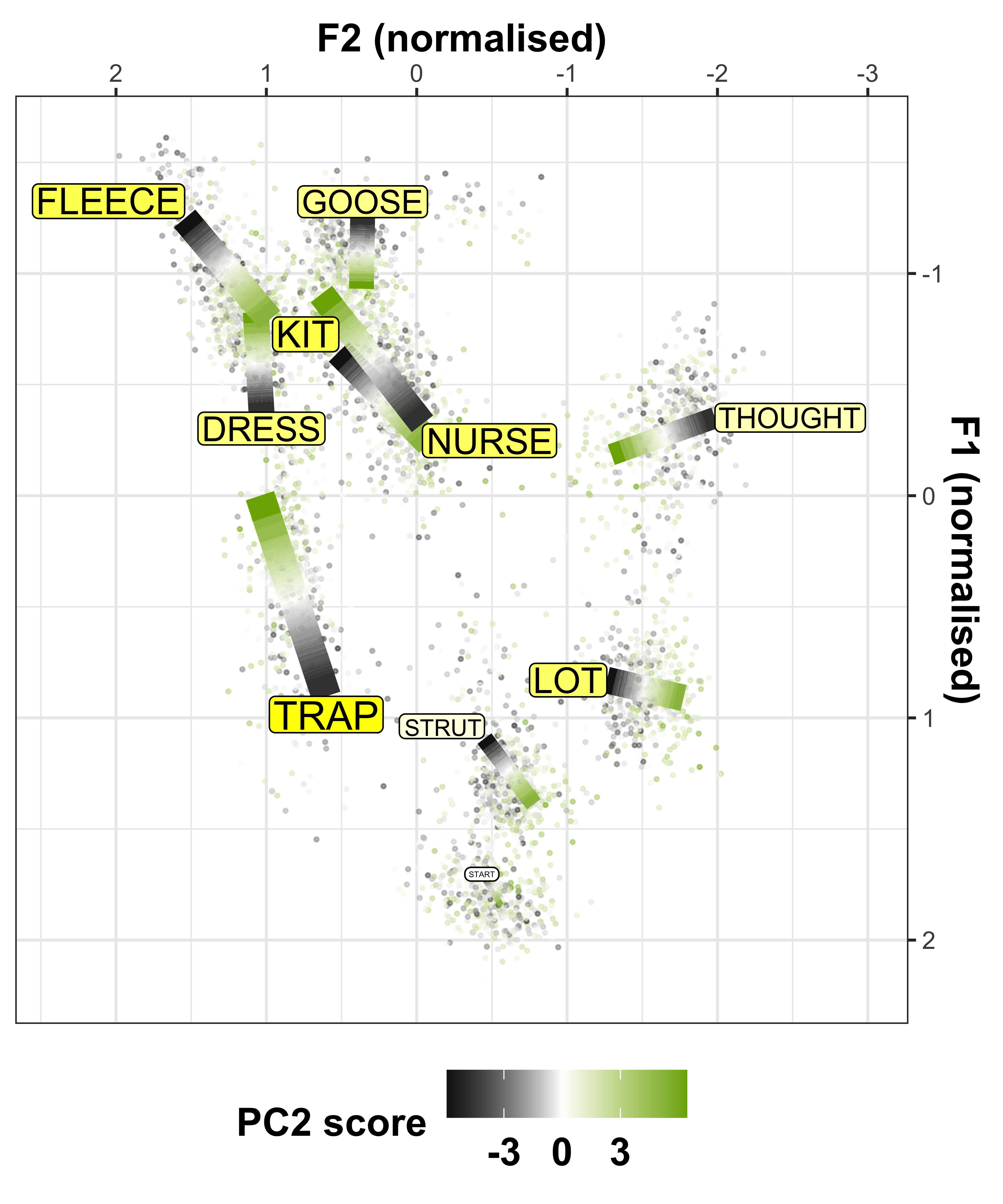

ggsave(plot = mod_pred_PC2_values_vowel_plot, filename = "Figures/mod_pred_PC2_values_vowel_plot.png", width = 7, height = 7, dpi = 400)

mod_pred_PC3_values_vowel_plot <- mod_pred_PC3_values_plot %>%
  ggplot(aes(x = fitted.values1_F2, y = fitted.values1_F1, colour = -Comp.3, size = PC3_loading_max, group = Vowel)) +
  geom_point(aes(x = intercepts1_F2, y = intercepts1_F1), size = 0.4, alpha = 0.5) +
  # geom_path(data = mod_pred_PC3_values_plot %>% arrange(Vowel, participant_year_of_birth), aes(x = fit_F2, y = fit_F1, group = Vowel), size = 1, colour = "red") +
  geom_line() +
  geom_label(data = mod_pred_PC3_values_plot %>%
  mutate(fitted.values2_F1 = ifelse(Vowel %in% c("STRUT", "LOT", "THOUGHT"), 1,
                                    ifelse(Vowel %in% c("GOOSE", "START"), 0, 0.5)),
         fitted.values2_F2 = ifelse(Vowel %in% c("GOOSE", "NURSE", "KIT"), 1,
                                    ifelse(Vowel %in% c("FLEECE", "DRESS", "TRAP"), 0, 0.5))) %>%
               filter(-Comp.3 == min(-Comp.3)), aes(label = Vowel, fill = rescale(PC3_loading_max^2, to = c(0, 1)), vjust = fitted.values2_F1, hjust = fitted.values2_F2), label.padding = unit(0.1, "lines"), colour = "black", show.legend = FALSE) +
  xlab("F2 (normalised)") +
  ylab("F1 (normalised)") +
  scale_x_reverse(position = "top", limits = c(2.4, -3)) +
  scale_y_reverse(position = "right") +
  scale_colour_gradient2(name = "PC3 score", low = "black", mid = "white" , high = "#7CAE00",
                         midpoint=0, breaks = c(-3, 0, 3)) +
  scale_fill_gradient(low = "white", high = "yellow", guide = "none") +
  scale_size_continuous(range = c(1, 5), guide = "none") +
  # facet_wrap(~Vowel) +
  theme_bw() +
  theme(legend.position = "bottom", axis.title = element_text(size = 14, face = "bold"), legend.title = element_text(size = 14, face = "bold"), legend.text = element_text(size = 14, face = "bold"))

mod_pred_PC3_values_vowel_plot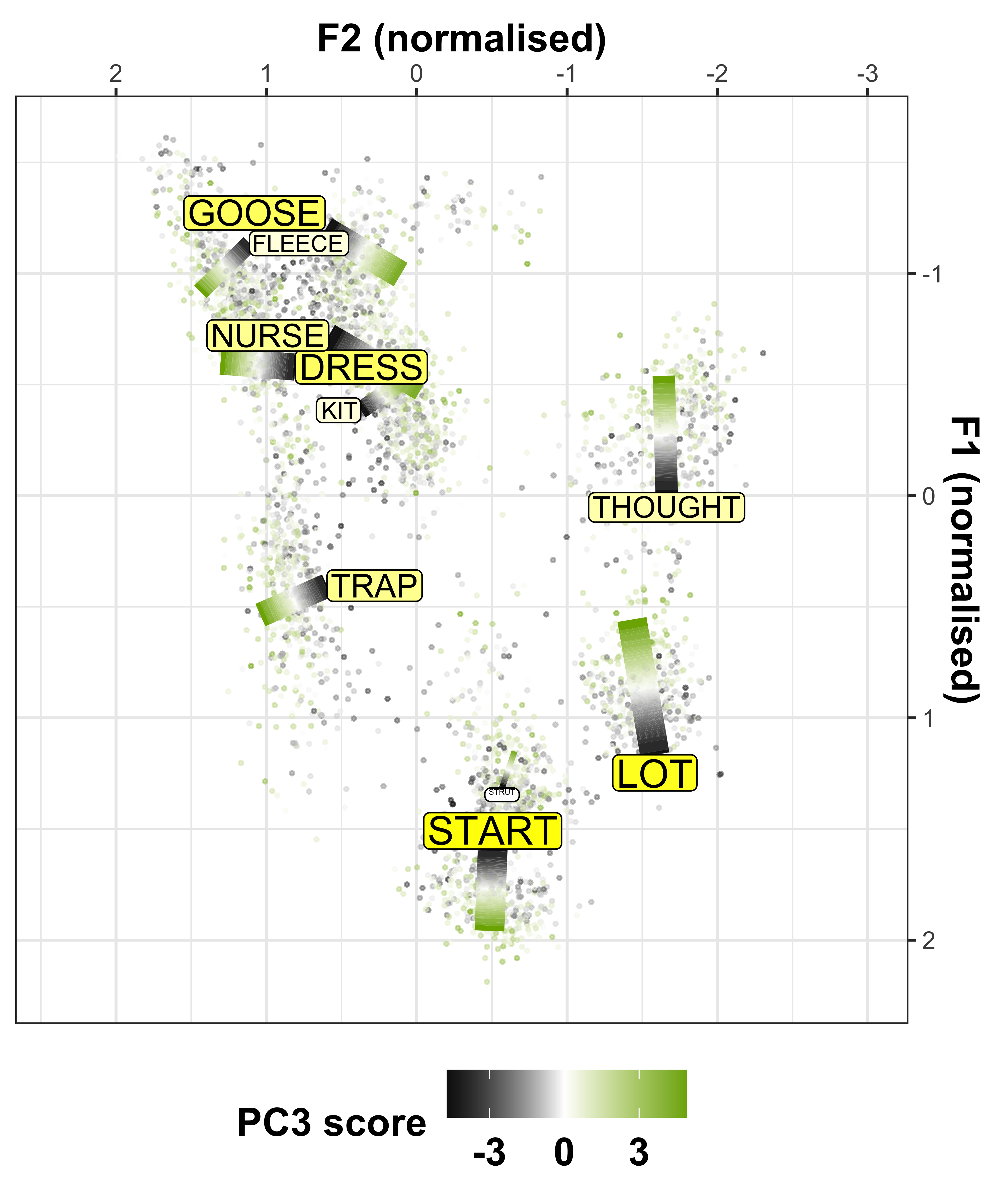

ggsave(plot = mod_pred_PC3_values_vowel_plot, filename = "Figures/mod_pred_PC3_values_vowel_plot.png", width = 7, height = 7, dpi = 400)

Relationship to sound change

Finally, we also want to see how the speaker intercepts and PC scores relate to sound change.

mod_pred_PC1_values_grid_plot <- mod_pred_PC1_values_plot %>%
           ungroup() %>%
  pivot_longer(intercepts_F1:intercepts_F2, names_to = "Formant", values_to = "intercepts") %>%
  mutate(Formant = substr(Formant, nchar(Formant)-1, nchar(Formant))) %>%
  left_join(mod_pred_PC1_values_plot %>%
              select(-intercepts_F1, -intercepts_F2) %>%
              pivot_longer(fit_F1:fit_F2, names_to = "Formant", values_to = "fit") %>%
              mutate(Formant = substr(Formant, nchar(Formant)-1, nchar(Formant)))) %>%
  left_join(mod_pred_PC1_values_plot %>%
              select(-intercepts_F1, -intercepts_F2, -fit_F1, -fit_F2) %>%
              pivot_longer(fitted.values_F1:fitted.values_F2, names_to = "Formant", values_to = "fitted.values") %>%
              mutate(Formant = substr(Formant, nchar(Formant)-1, nchar(Formant)))) %>%
  arrange(Vowel, abs(-Comp.1)) %>%
  ggplot(aes(x = participant_year_of_birth, colour = -Comp.1)) +
  geom_point(aes(y = intercepts + fit, size = abs(-Comp.1))) +
  # geom_point(aes(y = intercepts + fit), size = 1) +
  geom_path(data = gam_intercepts.tmp_long1 %>% arrange(Vowel, participant_year_of_birth), aes(y = fit, group = Vowel), size = 1, colour = "red") +
  geom_label(data = gam_intercepts.tmp_long1 %>% select(Vowel, Formant, PC1_loading) %>% distinct(), aes(x = ((max(vowels_all$participant_year_of_birth)-min(vowels_all$participant_year_of_birth))/2)+min(vowels_all$participant_year_of_birth), y = 2.7, label = paste0(round(PC1_loading^2, 3)*100, "%"), fill = rescale(PC1_loading^2, to = c(0, 1))), hjust = 0.5, inherit.aes = FALSE, show.legend = FALSE) +
  scale_x_continuous(name = "Participant year of birth", breaks = c(1900, 1950), limits = c(1856, 1990)) +
  scale_y_continuous(name = "Normalised formant value", breaks = c(-2, -1, 0, 1, 2), limits = c(-2.7, 3)) +
  # ylab("Normalised formant value") +
  scale_size_continuous(range = c(0.5, 1), guide = NULL) +
  scale_colour_gradient2(name = "PC1 score", low = "black", mid = "white" , high = "#7CAE00",
                         midpoint=0, breaks = c(-3, 0, 3)) +
  scale_fill_gradient(low = "white", high = "yellow") +
  geom_rect(data = gam_intercepts.tmp_long1_test %>% filter(Comp == "Comp.1" & highlight == "black"), aes(xmin = -Inf, xmax = Inf, ymin = -Inf, ymax = Inf), size = 5, alpha = 0, colour = "yellow") +
  facet_grid(factor(Formant, levels = c("F2", "F1"), ordered = TRUE)~Vowel) +
  theme_bw() +
  theme(legend.position = "none", axis.text = element_text(size = 12), axis.title = element_text(size = 14, face = "bold"), strip.text = element_text(size = 12, face = "bold"))

mod_pred_PC1_values_grid_plot

ggsave(plot = mod_pred_PC1_values_grid_plot, filename = "Figures/mod_pred_PC1_values_grid_plot.png", width = 12, height = 7, dpi = 400)

mod_pred_PC2_values_grid_plot <- mod_pred_PC2_values_plot %>%
           ungroup() %>%
  pivot_longer(intercepts_F1:intercepts_F2, names_to = "Formant", values_to = "intercepts") %>%
  mutate(Formant = substr(Formant, nchar(Formant)-1, nchar(Formant))) %>%
  left_join(mod_pred_PC2_values_plot %>%
              select(-intercepts_F1, -intercepts_F2) %>%
              pivot_longer(fit_F1:fit_F2, names_to = "Formant", values_to = "fit") %>%
              mutate(Formant = substr(Formant, nchar(Formant)-1, nchar(Formant)))) %>%
  left_join(mod_pred_PC2_values_plot %>%
              select(-intercepts_F1, -intercepts_F2, -fit_F1, -fit_F2) %>%
              pivot_longer(fitted.values_F1:fitted.values_F2, names_to = "Formant", values_to = "fitted.values") %>%
              mutate(Formant = substr(Formant, nchar(Formant)-1, nchar(Formant)))) %>%
  arrange(Vowel, abs(-Comp.2)) %>%
  ggplot(aes(x = participant_year_of_birth, colour = -Comp.2)) +
  geom_point(aes(y = intercepts + fit, size = abs(-Comp.2))) +
  # geom_point(aes(y = intercepts + fit), size = 1) +
  geom_path(data = gam_intercepts.tmp_long1 %>% arrange(Vowel, participant_year_of_birth), aes(y = fit, group = Vowel), size = 1, colour = "red") +
  geom_label(data = gam_intercepts.tmp_long1 %>% select(Vowel, Formant, PC2_loading) %>% distinct(), aes(x = ((max(vowels_all$participant_year_of_birth)-min(vowels_all$participant_year_of_birth))/2)+min(vowels_all$participant_year_of_birth), y = 2.7, label = paste0(round(PC2_loading^2, 3)*100, "%"), fill = rescale(PC2_loading^2, to = c(0, 1))), hjust = 0.5, inherit.aes = FALSE, show.legend = FALSE) +
  scale_x_continuous(name = "Participant year of birth", breaks = c(1900, 1950), limits = c(1856, 1990)) +
  scale_y_continuous(name = "Normalised formant value", breaks = c(-2, -1, 0, 1, 2), limits = c(-2.7, 3)) +
  # ylab("Normalised formant value") +
  scale_size_continuous(range = c(0.5, 1), guide = NULL) +
  scale_colour_gradient2(name = "PC2 score", low = "black", mid = "white" , high = "#7CAE00",
                         midpoint=0, breaks = c(-3, 0, 3)) +
  scale_fill_gradient(low = "white", high = "yellow") +
  geom_rect(data = gam_intercepts.tmp_long1_test %>% filter(Comp == "Comp.2" & highlight == "black"), aes(xmin = -Inf, xmax = Inf, ymin = -Inf, ymax = Inf), size = 5, alpha = 0, colour = "yellow") +
  facet_grid(factor(Formant, levels = c("F2", "F1"), ordered = TRUE)~Vowel) +
  theme_bw() +
  theme(legend.position = "none", axis.text = element_text(size = 12), axis.title = element_text(size = 14, face = "bold"), strip.text = element_text(size = 12, face = "bold"))

mod_pred_PC2_values_grid_plot

ggsave(plot = mod_pred_PC2_values_grid_plot, filename = "Figures/mod_pred_PC2_values_grid_plot.png", width = 12, height = 7, dpi = 400)

mod_pred_PC3_values_grid_plot <- mod_pred_PC3_values_plot %>%
           ungroup() %>%
  pivot_longer(intercepts_F1:intercepts_F2, names_to = "Formant", values_to = "intercepts") %>%
  mutate(Formant = substr(Formant, nchar(Formant)-1, nchar(Formant))) %>%
  left_join(mod_pred_PC3_values_plot %>%
              select(-intercepts_F1, -intercepts_F2) %>%
              pivot_longer(fit_F1:fit_F2, names_to = "Formant", values_to = "fit") %>%
              mutate(Formant = substr(Formant, nchar(Formant)-1, nchar(Formant)))) %>%
  left_join(mod_pred_PC3_values_plot %>%
              select(-intercepts_F1, -intercepts_F2, -fit_F1, -fit_F2) %>%
              pivot_longer(fitted.values_F1:fitted.values_F2, names_to = "Formant", values_to = "fitted.values") %>%
              mutate(Formant = substr(Formant, nchar(Formant)-1, nchar(Formant)))) %>%
  arrange(Vowel, abs(-Comp.3)) %>%
  ggplot(aes(x = participant_year_of_birth, colour = -Comp.3)) +
  geom_point(aes(y = intercepts + fit, size = abs(-Comp.3))) +
  # geom_point(aes(y = intercepts + fit), size = 1) +
  geom_path(data = gam_intercepts.tmp_long1 %>% arrange(Vowel, participant_year_of_birth), aes(y = fit, group = Vowel), size = 1, colour = "red") +
  # geom_smooth(aes(x = rescale(-Comp.3, to = c(min(participant_year_of_birth), max(participant_year_of_birth))), y = intercepts), method = "lm") +
  geom_label(data = gam_intercepts.tmp_long1 %>% select(Vowel, Formant, PC3_loading) %>% distinct(), aes(x = ((max(vowels_all$participant_year_of_birth)-min(vowels_all$participant_year_of_birth))/2)+min(vowels_all$participant_year_of_birth), y = 2.7, label = paste0(round(PC3_loading^2, 3)*100, "%"), fill = rescale(PC3_loading^2, to = c(0, 1))), hjust = 0.5, inherit.aes = FALSE, show.legend = FALSE) +
  scale_x_continuous(name = "Participant year of birth", breaks = c(1900, 1950), limits = c(1856, 1990)) +
  scale_y_continuous(name = "Normalised formant value", breaks = c(-2, -1, 0, 1, 2), limits = c(-2.7, 3)) +
  # ylab("Normalised formant value") +
  scale_size_continuous(range = c(0.5, 1), guide = NULL) +
  scale_colour_gradient2(name = "PC3 score", low = "black", mid = "white" , high = "#7CAE00",
                         midpoint=0, breaks = c(-3, 0, 3)) +
  scale_fill_gradient(low = "white", high = "yellow") +
  geom_rect(data = gam_intercepts.tmp_long1_test %>% filter(Comp == "Comp.3" & highlight == "black"), aes(xmin = -Inf, xmax = Inf, ymin = -Inf, ymax = Inf), size = 5, alpha = 0, colour = "yellow") +
  facet_grid(factor(Formant, levels = c("F2", "F1"), ordered = TRUE)~Vowel) +
  theme_bw() +
  theme(legend.position = "none", axis.text = element_text(size = 12), axis.title = element_text(size = 14, face = "bold"), strip.text = element_text(size = 12, face = "bold"))

mod_pred_PC3_values_grid_plot

ggsave(plot = mod_pred_PC3_values_grid_plot, filename = "Figures/mod_pred_PC3_values_grid_plot.png", width = 12, height = 7, dpi = 400)

Combine the plots

PC1_variables_combined_plot1 <- plot_grid(PC1_contrib_plot, NULL, rel_heights = c(1, 0.1), nrow = 2, ncol = 1)

PC1_variables_combined_plot <- plot_grid(NULL, plot_grid(NULL, NULL, labels = c("A", "B"), label_size = 25), plot_grid(PC1_variables_combined_plot1, mod_pred_PC1_values_vowel_plot, align = "vh", axis = "t"), nrow = 3, rel_heights = c(0.1, 0.08, 1), labels = c("PC1", "", ""), label_size = 25, label_x = -0.015, align = "hv")

# ggsave(plot = PC1_variables_combined_plot, filename = "Figures/PC1_plot_variables_combined.png", width = 14, height = 7, dpi = 600)

PC2_variables_combined_plot1 <- plot_grid(PC2_contrib_plot, NULL, rel_heights = c(1, 0.1), nrow = 2, ncol = 1)

PC2_variables_combined_plot <- plot_grid(NULL, plot_grid(NULL, NULL, labels = c("A", "B"), label_size = 25), plot_grid(PC2_variables_combined_plot1, mod_pred_PC2_values_vowel_plot, align = "vh", axis = "t"), nrow = 3, rel_heights = c(0.1, 0.08, 1), labels = c("PC2", "", ""), label_size = 25, label_x = -0.015, align = "hv")

# ggsave(plot = PC2_variables_combined_plot, filename = "Figures/PC2_plot_variables_combined.png", width = 14, height = 7, dpi = 600)

PC3_variables_combined_plot1 <- plot_grid(PC3_contrib_plot, NULL, rel_heights = c(1, 0.1), nrow = 2, ncol = 1)

PC3_variables_combined_plot <- plot_grid(NULL, plot_grid(NULL, NULL, labels = c("A", "B"), label_size = 25), plot_grid(PC3_variables_combined_plot1, mod_pred_PC3_values_vowel_plot, align = "vh", axis = "t"), nrow = 3, rel_heights = c(0.1, 0.08, 1), labels = c("PC3", "", ""), label_size = 25, label_x = -0.015, align = "hv")

# ggsave(plot = PC3_variables_combined_plot, filename = "Figures/PC3_plot_variables_combined.png", width = 14, height = 7, dpi = 600)

PC1_plot_combined <- plot_grid(PC1_variables_combined_plot, NULL, mod_pred_PC1_values_grid_plot, rel_heights = c(1, 0.08, 1), labels = c("", "C", ""), label_size = 25, nrow = 3)

PC1_plot_combined

ggsave(plot = PC1_plot_combined, filename = "Figures/PC1_plot.png", width = 15, height = 15, dpi = 600)

PC2_plot_combined <- plot_grid(PC2_variables_combined_plot, mod_pred_PC2_values_grid_plot, labels = c("", "C"), label_size = 25, nrow = 2)

PC2_plot_combined

ggsave(plot = PC2_plot_combined, filename = "Figures/PC2_plot.png", width = 15, height = 15, dpi = 600)

PC3_plot_combined <- plot_grid(PC3_variables_combined_plot, mod_pred_PC3_values_grid_plot, labels = c("", "C"), label_size = 25, nrow = 2)

PC3_plot_combined

ggsave(plot = PC3_plot_combined, filename = "Figures/PC3_plot.png", width = 15, height = 15, dpi = 600)

PCs combined

To understand which variables are linked to each other in terms of vowel space, we can visualise all 3 PCs on one plot, connecting the variables together by lines depending on which PC the variable is linked to. This highlights the point that no vowel is independent of others within the system.

#transform data so there are separate columns for F1 and F2
sound_change_plot_data1 <- mod_pred_yob_values %>%
  select(participant_year_of_birth, fit, Vowel, Formant) %>%
  pivot_wider(names_from = Formant, values_from = fit) %>% #transform the data to wide format so there are separate F1 and F2 variables
  mutate(PC1 = ifelse(Vowel %in% c("START", "STRUT", "THOUGHT"), TRUE, FALSE),
         PC2 = ifelse(Vowel %in% c("DRESS", "LOT", "NURSE", "FLEECE", "KIT", "TRAP"), TRUE, FALSE),
         PC3 = ifelse(Vowel %in% c("DRESS", "GOOSE", "LOT", "START"), TRUE, FALSE))

#make data frame to plot starting point, this will give the vowel labels based on the smallest year of birth coordinates
sound_change_labels1 <- sound_change_plot_data1 %>%
  group_by(Vowel) %>%
  filter(participant_year_of_birth == min(participant_year_of_birth)) %>%
  mutate(F2 = ifelse(Vowel == "DRESS", 1.25,
                     ifelse(Vowel == "LOT", -1.5,
                            ifelse(Vowel == "KIT", F2 - 0.25, F2))),
         F1 = ifelse(Vowel %in% c("DRESS", "NURSE", "THOUGHT", "LOT", "STRUT"), F1 - 0.4,
                     ifelse(Vowel == "TRAP", F1 - 0.6,
                            ifelse(Vowel == "KIT", F1 -0.2,
                                   ifelse(Vowel == "START", F1 + 0.02, F1))))) %>%
  ungroup()

hull_PC1 <- sound_change_labels1 %>%
  filter(PC1 == TRUE) %>%
  # select(Vowel, F2, F1) %>%
  distinct() %>%
  slice(chull(F1, F2)) %>%
  mutate(PC = "PC1") %>%
  as.data.frame()

hull_PC2 <- sound_change_labels1 %>%
  filter(PC2 == TRUE) %>%
  distinct() %>%
  slice(chull(F1, F2)) %>%
  mutate(PC = "PC2") %>%
  as.data.frame()

hull_PC3 <- sound_change_labels1 %>%
  filter(PC3 == TRUE) %>%
  # select(Vowel, F2, F1) %>%
  distinct() %>%
  slice(chull(F1, F2)) %>%
  mutate(PC = "PC3") %>%
  as.data.frame()

hulls <- rbind(hull_PC1, head(hull_PC1, 1), hull_PC2, head(hull_PC2, 1), hull_PC3, head(hull_PC3, 1)) %>%
  left_join(sound_change_labels1 %>% rename(F1_label = F1, F2_label = F2))

#plot
PC_hull_plot <- hulls %>%
  ggplot() +
  geom_path(aes(x = F2, y = F1, linetype = PC), colour = "black", alpha = 1, fill=NA, show.legend = TRUE) +
  geom_label(aes(x = F2_label, y = F1_label, label = Vowel), colour = "white", fill = "white", lwd = NA, show.legend = FALSE) +
  geom_text(aes(x = F2_label, y = F1_label, colour = Vowel, label = Vowel), show.legend = FALSE) +
  #label the axes
  xlab("F2 (normalised)") +
  ylab("F1 (normalised)") +
  #scale the size so the path is not too wide
  scale_size_continuous(range = c(0.2,1)) +
  #reverse the axes to follow conventional vowel plotting
  scale_x_reverse(limits = c(2,-2), position = "top") +
  scale_y_reverse(limits = c(2,-2), position = "right") +
  #set the colours
  scale_color_manual(values = c("#9590FF", "#D89000", "#A3A500", "#39B600", "#00BF7D",
                                 "#00BFC4", "#00B0F6", "#F8766D", "#E76BF3", "#FF62BC")) +
  scale_linetype_manual(values = c(1, 5, 3)) +
  #set the theme
  theme_bw() +
  #make title bold
  theme(plot.title = element_text(face="bold"),
        legend.position = c(0.87, 0.9),
        # legend.background = element_rect(colour = 'black', fill = 'white', linetype='solid'),
        legend.title = element_blank()) +
  guides(linetype=guide_legend(keywidth = 2.5, keyheight = 1, label.position = "left"),
         colour=guide_colorbar("none"))

PC_hull_plot

ggsave(plot = PC_hull_plot, filename = "Figures/summary_PC.png", width = 5.5, height = 5.5, dpi = 300)

PC scores and year of birth

Next, our analyses will inspect whether the PC scores within each of the 3 PCs are independent of social information, i.e. year of birth and gender.

We will begin by running GAMs to see if any of the socio-demographic variables can predict the PC scores significantly.

We hypothesise that our initial GAMMs had these variables included in the fixed-effects structure, so, none of the subsequent models should show significant results. If there are no significant effects, then we have confidence in our modelling procedure and that the speaker intercepts are representative of variation independent of the known predictors of change in F1/F2.

In order to statistically assess whether the PC scores are reliably predicted by any of the social variables, we will run a series of GAMs, predicting the PC scores in each of the 3 PCs by each of the social variables. We will also provide visualisations of the results.

PC1

#run a GAM to predict the PCA score on PC1 by the social information
# (entering Gender as a factor here (not ordered!), which generates
#  completely separate smooths for each Gender)
gam_PC1 = bam(-Comp.1 ~
             s(participant_year_of_birth, k=10, by=Gender) +
             Gender +
             Corpus,
           data=PC_speaker_loadings)

summary(gam_PC1)

## 
## Family: gaussian 
## Link function: identity 
## 
## Formula:
## -Comp.1 ~ s(participant_year_of_birth, k = 10, by = Gender) + 
##     Gender + Corpus
## 
## Parametric coefficients:
##                Estimate Std. Error t value Pr(>|t|)   
## (Intercept)     0.04203    0.13690   0.307  0.75899   
## GenderM        -0.04773    0.17182  -0.278  0.78129   
## CorpusDarfield -1.09406    0.38502  -2.842  0.00468 **
## CorpusIA        0.03169    0.29025   0.109  0.91311   
## CorpusMU        0.38015    0.41250   0.922  0.35722   
## ---
## Signif. codes:  0 '***' 0.001 '**' 0.01 '*' 0.05 '.' 0.1 ' ' 1
## 
## Approximate significance of smooth terms:
##                                      edf Ref.df     F p-value
## s(participant_year_of_birth):GenderM   1      1 0.482   0.488
## 
## R-sq.(adj) =  0.00986   Deviance explained = 2.02%
## fREML = 979.42  Scale est. = 3.4209    n = 481

# extract predictions
gam_PC1_preds <- plot_smooth(gam_PC1, view="participant_year_of_birth", plot_all="Gender")$fv

## Summary:
##  * Gender : factor; set to the value(s): F, M. 
##  * Corpus : factor; set to the value(s): CC. 
##  * participant_year_of_birth : numeric predictor; with 30 values ranging from 1864.000000 to 1982.000000. 
##  * NOTE : No random effects in the model to cancel.
## 

PC1_speaker_loadings <- ggplot(PC_speaker_loadings, aes(x = participant_year_of_birth, y = -Comp.1, #plot year of birth on the x axis and PC2 score on the y axis
                                label = Gender, color = Gender)) + #make the colours and data points represent Gender
  geom_point(size = 0, stroke = 0, show.legend = FALSE) + #add an empty data point for plotting
  geom_text(show.legend = FALSE) + #add text label i.e. F/M
  geom_ribbon(data=gam_PC1_preds, aes(ymin=-ll, ymax=-ul, y=NULL, group = Gender), col="grey", alpha = 0.2) +
  geom_line(data=gam_PC1_preds, aes(y=-fit), size = 1.25) +
  scale_y_continuous(breaks = seq(-6,6,2), limits = c(-7,7)) +
  scale_color_manual(breaks = c("F", "M"), labels = c("Female", "Male"), values = c("black", "#7CAE00")) + #update the legend and colour scheme where F = black letters, M = green letters
  scale_fill_manual(breaks = c("F", "M"), values = c("black", "#7CAE00"), guide=F) + #update the legend and colour scheme where F = black letters, M = green letters
  xlab("Year of birth") + #label x axis
  ylab("PC1 score") + #label y axis
  theme_bw() + #general aesthetics
  theme(axis.text = element_text(face = "bold", size = 14), axis.title = element_text(face = "bold", size = 14), legend.position = "none") #make the text bold and larger on the axes

PC1_speaker_loadings

# ggsave(plot = PC1_speaker_loadings, filename = "Figures/PC1_speaker_loadings.png", width = 7, height = 3, dpi = 300)

PC2

#run a GAM to predict the PCA score on PC1 by the social information
# (entering Gender as a factor here (not ordered!), which generates
#  completely separate smooths for each Gender)
gam_PC2 = bam(-Comp.2 ~
             s(participant_year_of_birth, k=10, by=Gender) +
             Gender +
             Corpus,
           data=PC_speaker_loadings)

summary(gam_PC2)

## 
## Family: gaussian 
## Link function: identity 
## 
## Formula:
## -Comp.2 ~ s(participant_year_of_birth, k = 10, by = Gender) + 
##     Gender + Corpus
## 
## Parametric coefficients:
##                Estimate Std. Error t value Pr(>|t|)
## (Intercept)     0.06671    0.13198   0.505    0.613
## GenderM         0.01742    0.16565   0.105    0.916
## CorpusDarfield -0.45667    0.37118  -1.230    0.219
## CorpusIA       -0.11459    0.27981  -0.410    0.682
## CorpusMU       -0.40713    0.39768  -1.024    0.306
## 
## Approximate significance of smooth terms:
##                                      edf Ref.df     F p-value
## s(participant_year_of_birth):GenderM   1      1 0.579   0.447
## 
## R-sq.(adj) =  -0.00572   Deviance explained = 0.476%
## fREML = 962.04  Scale est. = 3.1794    n = 481

# extract predictions
gam_PC2_preds <- plot_smooth(gam_PC2, view="participant_year_of_birth", plot_all="Gender")$fv

## Summary:
##  * Gender : factor; set to the value(s): F, M. 
##  * Corpus : factor; set to the value(s): CC. 
##  * participant_year_of_birth : numeric predictor; with 30 values ranging from 1864.000000 to 1982.000000. 
##  * NOTE : No random effects in the model to cancel.
## 

#this code repeats the same process as in PC1, but for PC2
PC2_speaker_loadings <- ggplot(PC_speaker_loadings, aes(x = participant_year_of_birth, y = -Comp.2, #plot year of birth on the x axis and PC2 score on the y axis
                                label = Gender, color = Gender)) + #make the colours and data points represent Gender
  geom_point(size = 0, stroke = 0, show.legend = FALSE) + #add an empty data point for plotting
  geom_text(show.legend = FALSE) + #add text label i.e. F/M
  geom_ribbon(data=gam_PC2_preds, aes(ymin=-ll, ymax=-ul, y=NULL, group = Gender), col="grey", alpha = 0.2) +
  geom_line(data=gam_PC2_preds, aes(y=-fit), size = 1.25) +
  scale_y_continuous(breaks = seq(-6,6,2), limits = c(-7,7)) +
  scale_color_manual(breaks = c("F", "M"), labels = c("Female", "Male"), values = c("black", "#7CAE00")) + #update the legend and colour scheme where F = black letters, M = green letters
  scale_fill_manual(breaks = c("F", "M"), values = c("black", "#7CAE00"), guide=F) + #update the legend and colour scheme where F = black letters, M = green letters
  xlab("Year of birth") + #label x axis
  ylab("PC2 score") + #label y axis
  theme_bw() + #general aesthetics
  theme(axis.text = element_text(face = "bold", size = 14), axis.title = element_text(face = "bold", size = 14), legend.position = "none") #make the text bold and larger on the axes

PC2_speaker_loadings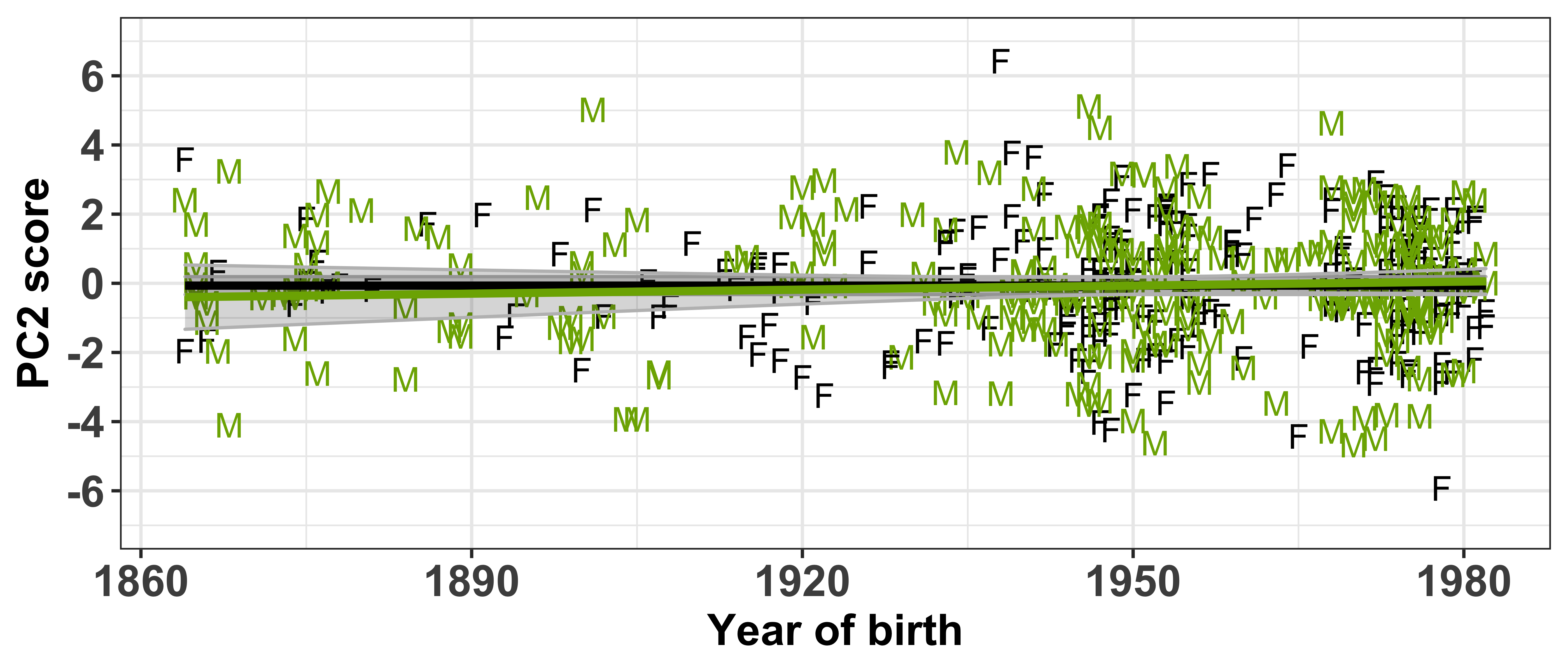

# ggsave(plot = PC2_speaker_loadings, filename = "Figures/PC2_speaker_loadings.png", width = 7, height = 3, dpi = 300)

PC3

#run a GAM to predict the PCA score on PC1 by the social information
# (entering Gender as a factor here (not ordered!), which generates
#  completely separate smooths for each Gender)
gam_PC3 = bam(-Comp.3 ~
             s(participant_year_of_birth, k=10, by=Gender) +
             Gender +
             Corpus,
           data=PC_speaker_loadings)

summary(gam_PC3)

## 
## Family: gaussian 
## Link function: identity 
## 
## Formula:
## -Comp.3 ~ s(participant_year_of_birth, k = 10, by = Gender) + 
##     Gender + Corpus
## 
## Parametric coefficients:
##                 Estimate Std. Error t value Pr(>|t|)    
## (Intercept)    -0.153924   0.099162  -1.552    0.121    
## GenderM         0.026154   0.124460   0.210    0.834    
## CorpusDarfield  2.261643   0.278891   8.109 4.37e-15 ***
## CorpusIA        0.002837   0.210242   0.013    0.989    
## CorpusMU        0.222118   0.298801   0.743    0.458    
## ---
## Signif. codes:  0 '***' 0.001 '**' 0.01 '*' 0.05 '.' 0.1 ' ' 1
## 
## Approximate significance of smooth terms:
##                                      edf Ref.df     F p-value
## s(participant_year_of_birth):GenderM   1      1 0.201   0.654
## 
## R-sq.(adj) =  0.114   Deviance explained = 12.3%
## fREML = 826.25  Scale est. = 1.7949    n = 481

# extract predictions
gam_PC3_preds <- plot_smooth(gam_PC3, view="participant_year_of_birth", plot_all="Gender")$fv

## Summary:
##  * Gender : factor; set to the value(s): F, M. 
##  * Corpus : factor; set to the value(s): CC. 
##  * participant_year_of_birth : numeric predictor; with 30 values ranging from 1864.000000 to 1982.000000. 
##  * NOTE : No random effects in the model to cancel.
## 

#this code repeats the same process as in PC1, but for PC2
PC3_speaker_loadings <- ggplot(PC_speaker_loadings, aes(x = participant_year_of_birth, y = -Comp.3, #plot year of birth on the x axis and PC3 score on the y axis
                                label = Gender, color = Gender)) + #make the colours and data points represent Gender
  geom_point(size = 0, stroke = 0, show.legend = FALSE) + #add an empty data point for plotting
  geom_text(show.legend = FALSE) + #add text label i.e. F/M
  geom_ribbon(data=gam_PC3_preds, aes(ymin=-ll, ymax=-ul, y=NULL, group = Gender), col="grey", alpha = 0.2) +
  geom_line(data=gam_PC3_preds, aes(y=-fit), size = 1.25) +
  scale_y_continuous(breaks = seq(-6,6,2), limits = c(-7,7)) +
  scale_color_manual(breaks = c("F", "M"), labels = c("Female", "Male"), values = c("black", "#7CAE00")) + #update the legend and colour scheme where F = black letters, M = green letters
  scale_fill_manual(breaks = c("F", "M"), values = c("black", "#7CAE00"), guide=F) + #update the legend and colour scheme where F = black letters, M = green letters
  xlab("Year of birth") + #label x axis
  ylab("PC3 score") + #label y axis
  theme_bw() + #general aesthetics
  theme(axis.text = element_text(face = "bold", size = 14), axis.title = element_text(face = "bold", size = 14), legend.position = "none") #make the text bold and larger on the axes

PC3_speaker_loadings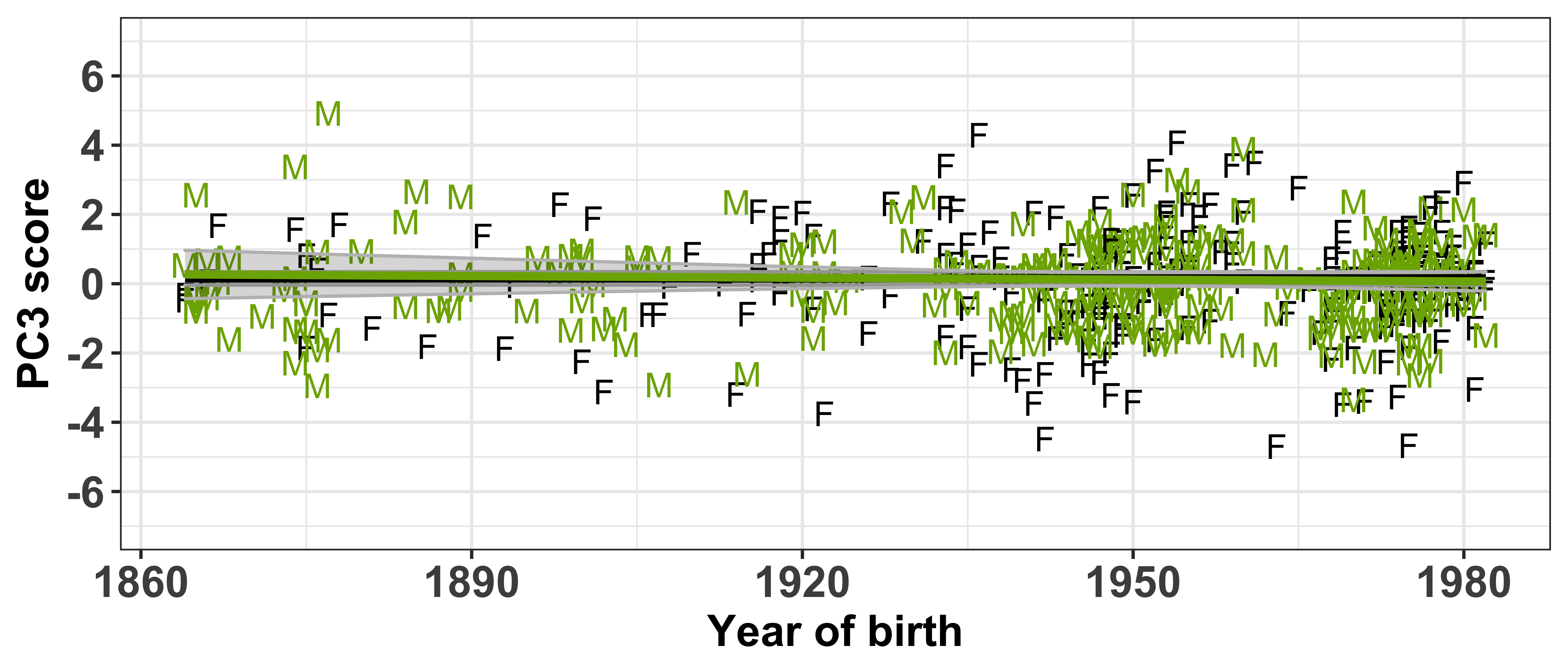

# ggsave(plot = PC3_speaker_loadings, filename = "Figures/PC3_speaker_loadings.png", width = 7, height = 3, dpi = 300)

Relationship between the PC scores

It may be of interest to inspect the how the PC scores correlate with each other, i.e. checking that if you have a high score on one PC does that predict a high score on the other PCs? The correlations below show that there is no strong trends to support this, demonstrating that the PC scores and the PCs are independent.

Note however, there does seem to be a slight trend for speakers with high PC1 to have high PC3.

chart.Correlation(PC_speaker_loadings %>% select(Comp.1:Comp.3), histogram = FALSE, pch=19)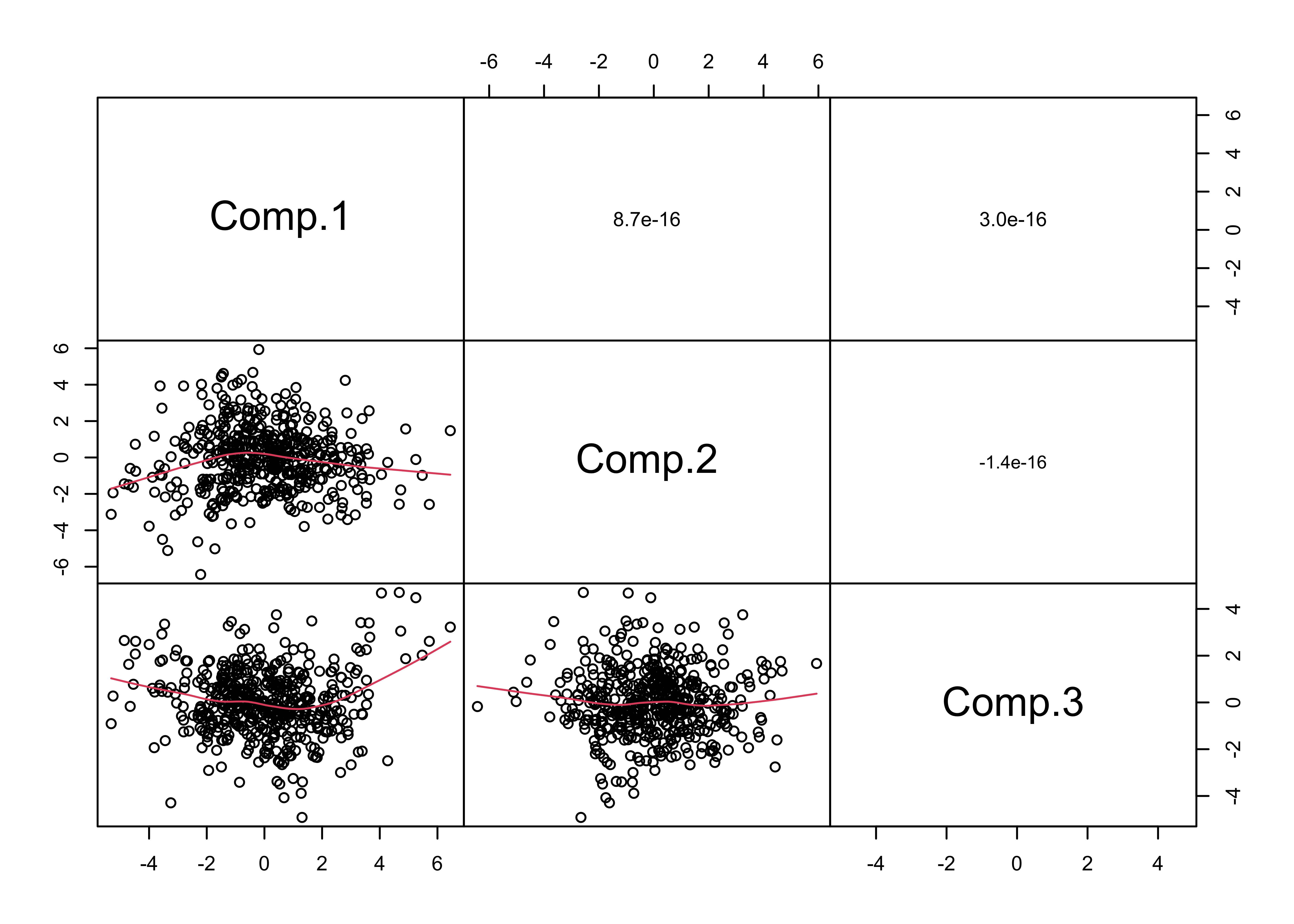

Additional analyses

Mixed-effects modelling

An alternative approach to obtaining the speaker intercepts would be to use linear mixed-effects modelling. This is done using the lme4 package, if you are unfamiliar with this form of regression analysis, an introductory tutorial Winter, 2013 can be found here for part 1 and here for part 2, for further information about why we chose the by-speaker intercepts, please refer to the manuscript or see Drager and Hay (2012)

We will generate the intercepts and visually see if there is a strong linear relationship between the intercepts generated from the GAMMs.

Note, this was our original approach taken to the analysis, we decided however that the GAMMs were the most suitable approach given our dataset. We include the following code below for those interested in using linear mixed-effects models.

Fitting procedure

The fitting procedure is identical to that used in the GAMMs analysis.

All models will be fit uniformly, i.e. with the same fixed and random effects structures (note, we model the year of birth variable non-linearly, this is done with a restricted cubic spline with 4 knots, see here for more information about what this means).

Note this process takes ~4 minutes to complete.

#create a data frame to store the intercepts from the models, this will initially contain just the speaker names
lmer_intercepts.tmp <- vowels_all %>%
  select(Speaker) %>%
  arrange(Speaker) %>%
  distinct()

#loop through the vowels

for (i in levels(factor(vowels_all$Vowel))) {

  cat(paste0(i, ": ", format(Sys.time(), "%d %B %Y, %r"), " ✅\n"))  #print the vowel the loop is up to

  #run the mixed-effects model on the vowel, i.e. if i = FLEECE this will model F1 for FLEECE
  lmer.F1 <- lmer(F1_lobanov_2.0 ~
                  scale(rcs(participant_year_of_birth, 4))*Gender +
                  Speech_rate +
                  (1|Speaker) +
                  (1|Word),
                data = vowels_all,
                subset = Vowel == i)

  #extract the speaker intercepts from the model and store them in a temporary data frame
  lmer.F1.intercepts.tmp <- ranef(lmer.F1)[["Speaker"]]

  #run the mixed-effects model on the vowel, i.e. if i = FLEECE this will model F2 for FLEECE
  lmer.F2 <- lmer(F2_lobanov_2.0 ~
                  scale(rcs(participant_year_of_birth, 4))*Gender +
                  Speech_rate +
                  (1|Speaker) +
                  (1|Word),
                data = vowels_all,
                subset = Vowel == i)

  #extract the speaker intercepts again, storing them in a separate data frame
  lmer.F2.intercepts.tmp <- ranef(lmer.F2)[["Speaker"]]

  #rename the variables so it clear which one has F1/F2, i.e. this will give F1_FLEECE, F2_FLEECE
  names(lmer.F1.intercepts.tmp) <- paste0("F1_", i)
  names(lmer.F2.intercepts.tmp) <- paste0("F2_", i)

  #combine the intercepts for F1 and F2 and store them in the intercepts.tmp_stress data frame
  lmer_intercepts.tmp <- cbind(lmer_intercepts.tmp, lmer.F1.intercepts.tmp, lmer.F2.intercepts.tmp)
}

write.csv(lmer_intercepts.tmp, "Data/lmer_intercepts.csv", row.names = FALSE)

Load in the lmer intercepts

lmer_intercepts.tmp <- read.csv("Data/lmer_intercepts.csv")

Comparison with GAMMs

Visualise the GAMM intercepts with the lmer intercepts

lmer_intercepts.tmp_F1 <- lmer_intercepts.tmp %>%
  select(Speaker, contains("F1")) %>%
  pivot_longer(-Speaker, names_to = "F_variable", values_to = "F1_lmer_intercept") %>%
  mutate(Vowel = gsub("F1_", "", F_variable))

gam_intercepts.tmp_F1 <- gam_intercepts.tmp %>%
  select(Speaker, contains("F1")) %>%
  pivot_longer(-Speaker, names_to = "F_variable", values_to = "F1_GAMM_intercept") %>%
  mutate(Vowel = gsub("F1_", "", F_variable))

gam_intercepts.tmp_F1 %>%
  left_join(., lmer_intercepts.tmp_F1) %>%
  ggplot(aes(x = F1_GAMM_intercept, y = F1_lmer_intercept, colour = Vowel)) +
  geom_point(size = 0.5, show.legend = FALSE) +
  facet_wrap(~Vowel) +
  theme_bw()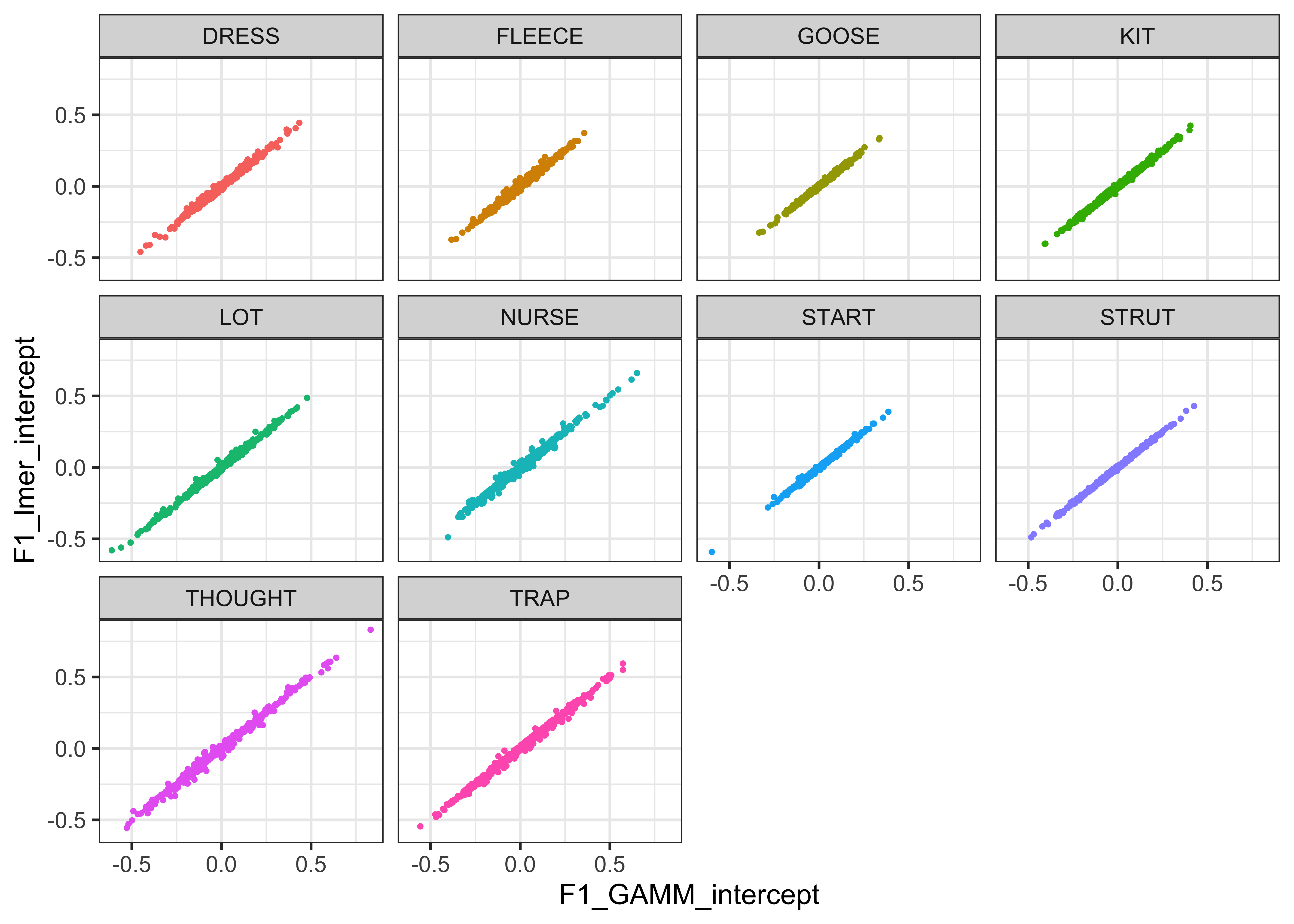

lmer_intercepts.tmp_F2 <- lmer_intercepts.tmp %>%
  select(Speaker, contains("F2")) %>%
  pivot_longer(-Speaker, names_to = "F_variable", values_to = "F2_lmer_intercept") %>%
  mutate(Vowel = gsub("F2_", "", F_variable))

gam_intercepts.tmp_F2 <- gam_intercepts.tmp %>%
  select(Speaker, contains("F2")) %>%
  pivot_longer(-Speaker, names_to = "F_variable", values_to = "F2_GAMM_intercept") %>%
  mutate(Vowel = gsub("F2_", "", F_variable))

gam_intercepts.tmp_F2 %>%
  left_join(., lmer_intercepts.tmp_F2) %>%
  ggplot(aes(x = F2_GAMM_intercept, y = F2_lmer_intercept, colour = Vowel)) +
  geom_point(size = 0.5, show.legend = FALSE) +
  facet_wrap(~Vowel) +
  theme_bw()

Ploting PCA by loading

An alternative to understanding how the variables contribute to each of the PCs is to look at the loadings. These are similiar to the % contribution values we present in the paper, they are widely used in PCA and the larger the absolute value (i.e. either positive or negative) then the more that variable contributes to the PC.

In the plots below, we present the absolute loading on the y axis, the red dashed line (which is located through y = square root of 0.05, approximately 0.224) gives the baseline where all loadings would be if they contributed equally to the PC.

PC1_loadings_plot <- ggplot(PC1_contrib, aes(x=reorder(Variable, Loading_abs), y=Loading_abs)) + #have the variable name on the x axis and loading value on the y
  geom_text(aes(alpha = highlight, label=ifelse(PC1_contrib$direction=="red","–", "+")), colour = PC1_contrib$direction, size = 6, fontface="bold", show.legend = FALSE) +
  xlab("") + #remove the x axis title
  ylab("PC1 loading (absolute)") +
  geom_hline(yintercept = sqrt(0.05), color = "red", linetype = "dashed") + #add a red dashed line to identify the 0.2 cut off
  scale_y_continuous(breaks = seq(0, 0.4, 0.1), limits = c(0, 0.4)) +
  scale_alpha_manual(values=c(1, 0.3)) +
  theme_bw() + #set the aesthetics of the plot
  theme(axis.text.x = element_text(angle = 90, hjust = 1, colour = PC1_contrib$highlight, size = 14, face = "bold"),
        axis.text.y = element_text(size = 14, face = "bold"),
        axis.title = element_text(size = 14, face = "bold")) #modify the x axis variable names so they are rotated and highlighted

PC2_loadings_plot <- ggplot(PC2_contrib, aes(x=reorder(Variable, Loading_abs), y=Loading_abs)) + #have the variable name on the x axis and loading value on the y
  geom_text(aes(alpha = highlight, label=ifelse(PC2_contrib$direction=="red","–", "+")), colour = PC2_contrib$direction, size = 6, fontface="bold", show.legend = FALSE) +
  xlab("") + #remove the x axis title
  ylab("PC2 loading (absolute)") +
  geom_hline(yintercept = sqrt(0.05), color = "red", linetype = "dashed") + #add a red dashed line to identify the 0.2 cut off
  scale_y_continuous(breaks = seq(0, 0.4, 0.1), limits = c(0, 0.4)) +
  scale_alpha_manual(values=c(1, 0.3)) +
  theme_bw() + #set the aesthetics of the plot
  theme(axis.text.x = element_text(angle = 90, hjust = 1, colour = PC2_contrib$highlight, size = 14, face = "bold"),
        axis.text.y = element_text(size = 14, face = "bold"),
        axis.title = element_text(size = 14, face = "bold")) #modify the x axis variable names so they are rotated and highlighted

PC3_loadings_plot <- ggplot(PC3_contrib, aes(x=reorder(Variable, Loading_abs), y=Loading_abs)) + #have the variable name on the x axis and loading value on the y
  geom_text(aes(alpha = highlight, label=ifelse(PC3_contrib$direction=="red","–", "+")), colour = PC3_contrib$direction, size = 6, fontface="bold", show.legend = FALSE) +
  xlab("") + #remove the x axis title
  ylab("PC3 loading (absolute)") +
  geom_hline(yintercept = sqrt(0.05), color = "red", linetype = "dashed") + #add a red dashed line to identify the 0.2 cut off
  scale_y_continuous(breaks = seq(0, 0.4, 0.1), limits = c(0, 0.4)) +
  scale_alpha_manual(values=c(1, 0.3)) +
  theme_bw() + #set the aesthetics of the plot
  theme(axis.text.x = element_text(angle = 90, hjust = 1, colour = PC3_contrib$highlight, size = 14, face = "bold"),
        axis.text.y = element_text(size = 14, face = "bold"),
        axis.title = element_text(size = 14, face = "bold")) #modify the x axis variable names so they are rotated and highlighted

#combine the 3 separate PC plots in to one
PC_loadings <- plot_grid(NULL, PC1_loadings_plot, PC2_loadings_plot, PC3_loadings_plot, labels = c("", "PC1 (17.2% variance)", "PC2 (15.8% variance)", "PC3 (10.1% variance)"), label_y = 1.04, rel_heights = c(0.1, 1, 1, 1), nrow = 4)

#view the plot
PC_loadings

ggsave(plot = plot_grid(NULL, PC1_loadings_plot, PC2_loadings_plot, PC3_loadings_plot, labels = c("", "PC1 (17.2% variance)", "PC2 (15.8% variance)", "PC3 (10.1% variance)"), label_x = -0.17, label_y = 1.05, rel_heights = c(0.1, 1, 1, 1), nrow = 4), filename = "Figures/PC_loadings.png", dpi = 600, height = 12, width = 5)

PCs by cumulative contribution

Another, more clear way to visualise how the variables contribute to the PCs is to show the cumulative proportions as the y axis variable. This is done to highlight that only a certain number of variables actually contribute a large amount of the explained variance. We will take a 50% cumulative contribution baseline to show which variables actually contribute a lot to each of the PCs.

PC1_loadings_contrib1 <- PC_loadings_contrib %>%
  filter(PC == "Loading.PC1") %>%
  arrange(Contribution.PC1) %>%
  # group_by(Variable) %>%
  mutate(cumsum_PC1 = round(cumsum(Contribution.PC1), 4),
         highlight = ifelse(cumsum_PC1 < 50, "grey", "black"),
         highlight1 = ifelse(cumsum_PC1 < 50, 0.5, 1),
         direction1 = direction,
         direction_lab = ifelse(direction1=="red","–", "+"))

PC1_loadings_contrib1_plot <- PC1_loadings_contrib1 %>%
  ggplot(aes(x = fct_reorder(Variable, cumsum_PC1), y = cumsum_PC1, label=direction_lab, colour = direction1)) +
  # geom_point() +
  geom_text(alpha = PC1_loadings_contrib1$highlight1, size = 6, fontface="bold", show.legend = FALSE) +
  scale_color_manual(values = c("black", "red")) +
  geom_vline(xintercept = 16.5, colour = "red", linetype = 2) +
  xlab("") +
  ylab("Cumulative sum contribution %\n(PC1)") +
  # facet_grid(PC~.) +
  theme_bw() +
  theme(axis.text.x = element_text(angle = 90, hjust = 1, colour = PC1_loadings_contrib1$highlight, size = 14, face = "bold")) #modify the x axis variable names so they are rotated and highlighted

PC2_loadings_contrib1 <- PC_loadings_contrib %>%
  filter(PC == "Loading.PC2") %>%
  arrange(Contribution.PC2) %>%
  # group_by(Variable) %>%
  mutate(cumsum_PC2 = round(cumsum(Contribution.PC2), 4),
         highlight = ifelse(cumsum_PC2 < 50, "grey", "black"),
         highlight1 = ifelse(cumsum_PC2 < 50, 0.5, 1),
         direction1 = direction,
         direction_lab = ifelse(direction1=="red","–", "+"))

PC2_loadings_contrib1_plot <- PC2_loadings_contrib1 %>%
  ggplot(aes(x = fct_reorder(Variable, cumsum_PC2), y = cumsum_PC2, label=direction_lab, colour = direction1)) +
  # geom_point() +
  geom_text(alpha = PC2_loadings_contrib1$highlight1, size = 6, fontface="bold", show.legend = FALSE) +
  scale_color_manual(values = c("black", "red")) +
  geom_vline(xintercept = 14.5, colour = "red", linetype = 2) +
  xlab("") +
  ylab("Cumulative sum contribution %\n(PC2)") +
  # facet_grid(PC~.) +
  theme_bw() +
  theme(axis.text.x = element_text(angle = 90, hjust = 1, colour = PC2_loadings_contrib1$highlight, size = 14, face = "bold")) #modify the x axis variable names so they are rotated and highlighted

PC3_loadings_contrib1 <- PC_loadings_contrib %>%
  filter(PC == "Loading.PC3") %>%
  arrange(Contribution.PC3) %>%
  # group_by(Variable) %>%
  mutate(cumsum_PC3 = round(cumsum(Contribution.PC3), 4),
         highlight = ifelse(cumsum_PC3 < 50, "grey", "black"),
         highlight1 = ifelse(cumsum_PC3 < 50, 0.5, 1),
         direction1 = direction,
         direction_lab = ifelse(direction1=="red","–", "+"))

PC3_loadings_contrib1_plot <- PC3_loadings_contrib1 %>%
  ggplot(aes(x = fct_reorder(Variable, cumsum_PC3), y = cumsum_PC3, label=direction_lab, colour = direction1)) +
  # geom_point() +
  geom_text(alpha = PC3_loadings_contrib1$highlight1, size = 6, fontface="bold", show.legend = FALSE) +
  scale_color_manual(values = c("black", "red")) +
  geom_vline(xintercept = 16.5, colour = "red", linetype = 2) +
  xlab("") +
  ylab("Cumulative sum contribution %\n(PC3)") +
  # facet_grid(PC~.) +
  theme_bw() +
  theme(axis.text.x = element_text(angle = 90, hjust = 1, colour = PC3_loadings_contrib1$highlight, size = 14, face = "bold")) #modify the x axis variable names so they are rotated and highlighted

PC_loadings_contrib1 <- plot_grid(NULL, PC1_loadings_contrib1_plot, NULL, PC2_loadings_contrib1_plot, NULL, PC3_loadings_contrib1_plot, labels = c("PC1", "", "PC2", "", "PC3", ""), rel_heights = c(0.2, 1, 0.2, 1, 0.2, 1), label_size = 14, nrow = 6)

PC_loadings_contrib1

# ggsave(plot = PC_loadings_contrib1, filename = "Figures/PC_loadings_contrib1.png", width = 6, height = 14, dpi = 300)

Previous PC scores analysis

Originally we modelled the PC scores based on GAMM models, where F1 and F2 values were predicted by the PC scores for each of the 3 PCs. We chose not to focus on this approach in the manuscript as PCA finds linear relationships, not non-linear relationships that GAMM models are suited to. We inlcude the following section for reference. The patterns are similar to the ones reported in the manuscript.

PC1

GAMM modelling

We will predict the F1 and F2 of each of the vowels again using GAMMs, with Comp.1 (the PCA scores for PC1) included as a smooth term. There are also random effects for Speaker and word.

These models are saved in the model_summaries folder for efficiency.

#loop through the vowels
for (i in levels(factor(vowels_all$Vowel))) {

  #F1 modelling
  cat(paste0("F1_", i, ": ", format(Sys.time(), "%d %B %Y, %r"), " ✅\n"))  #print the vowel the loop is up to for F1, as well as the start time for the model

  #run the mixed-effects model on the vowel, i.e. if i = FLEECE this will model F1 for FLEECE
  gam.F1 <- bam(F1_lobanov_2.0 ~
                  s(Comp.1, k = 10) +
                  s(Speaker, bs="re") +
                  s(Word, bs="re"),
                data=vowels_all %>% filter(Vowel == i),
                discrete=T, nthreads=2)

  #store the model
  assign(paste0("gam_F1_", i), gam.F1)

  #save the model summary
  saveRDS(gam.F1, file = paste0("/Users/james/Documents/GitHub/model_summaries/PC1/gam_F1_", i, ".rds"))

  #F2 modelling
  cat(paste0("F2_", i, ": ", format(Sys.time(), "%d %B %Y, %r"), " ✅\n")) #print the vowel the loop is up to for F2 , as well as the start time for the model

  #run the mixed-effects model on the vowel, i.e. if i = FLEECE this will model F2 for FLEECE
  gam.F2 <- bam(F2_lobanov_2.0 ~
                  s(Comp.1, k = 10) +
                  s(Speaker, bs="re") +
                  s(Word, bs="re"),
                data=vowels_all %>% filter(Vowel == i),
                discrete=T, nthreads=2)

  #store the model
  assign(paste0("gam_F2_", i), gam.F2)

  #save the model summary
  saveRDS(gam.F2, file = paste0("/Users/james/Documents/GitHub/model_summaries/PC1/gam_F2_", i, ".rds"))

}

Visualisation by GAM smooth

• x axis = PCA score

• y axis = normalised F1/F2

• smoothed lines = GAM fit

mod_pred_PC1_values <- readRDS("Data/Models/mod_pred_PC1_values.rds")

#get means for each speaker per vowel and formant
PC1_change_summary <- vowels_all %>%
  group_by(Speaker, Comp.1, Vowel) %>%
  dplyr::summarise(n = n(),
                   F1 = mean(F1_lobanov_2.0),
                   F2 = mean(F2_lobanov_2.0),
                   sd_F1 = sd(F1_lobanov_2.0),
                   sd_F2 = sd(F2_lobanov_2.0)) %>%
  ungroup() %>%
  pivot_longer(F1:F2, names_to = "Formant", values_to = "fit")

#plot the gam smooths predicting F1/F2 per vowel and add the per speaker mean values
PC1_plot_smooth <- mod_pred_PC1_values %>%
  mutate(Formant = factor(Formant, levels = c("F2", "F1"))) %>%
  ggplot(aes(x = -Comp.1, y = fit, colour = Formant, fill = Formant)) +
  geom_point(data = PC1_change_summary %>%
  mutate(Formant = factor(Formant, levels = c("F2", "F1"))), size = 0.25, alpha = 0.1) +
  geom_line(size = 1) +
  geom_ribbon(aes(ymin = ll, ymax = ul), alpha = 0.2, colour = NA) +
  scale_x_continuous(breaks = c(-4, 0, 4)) +
  xlab("PC1 score") +
  ylab("Predicted model fit (Lobanov 2.0)") +
  facet_grid(Formant~Vowel) +
  theme_bw() +
  theme(legend.position = "none", axis.text = element_text(size = 12), axis.title = element_text(size = 14, face = "bold"), strip.text = element_text(size = 12, face = "bold"))

PC1_plot_smooth

# ggsave(plot = PC1_plot_smooth, filename = "Figures/PC1_plot_gam.png", width = 10, height = 5, dpi = 300)

Visualisation in F1/F2 space

• x axis = F2

• y axis = F1

• colours = lexical set of vowel

• lines = trajectory of the F1/F2 in terms of PCA score (-5.5 to 6.5)

• vowel labels = start point of the vowel trajectory (smallest PCA score: -5.5)

• vowel label size = magnitude of variable loading, this is calculated from the dot plots from the original PCA, as there are 2 possible loadings (one for F1 and one for F2), the largest value is taken to represent the size

• arrows = end point of the trajectory (largest PCA score: 6.5)

#transform data so there are separate columns for F1 and F2
PC1_plot_data <- mod_pred_PC1_values %>%
  select(Comp.1, fit, Vowel, Formant) %>%
  mutate(Comp.1 = -Comp.1) %>%
  pivot_wider(names_from = Formant, values_from = fit) %>% #transform the data to wide format so there are separate F1 and F2 variables
  left_join(., PC1_loadings %>%
  group_by(Vowel) %>%
  filter(PC1_loadings_abs == max(PC1_loadings_abs)))

#make data frame to plot starting point, this will give the vowel labels based on the smallest PCA scores
PC1_change_labels1 <- PC1_plot_data %>%
  group_by(Vowel) %>%
  filter(Comp.1 == min(Comp.1))

#make data frame to plot end point, this will give the arrow at the end of the paths based on the largest year of birth coordinates
PC1_change_labels2 <- PC1_plot_data %>%
  group_by(Vowel) %>%
  top_n(wt = Comp.1, n = 2)

#plot
PC1_change_plot <- PC1_plot_data %>%
  mutate(PC1_loadings_abs = PC1_loadings_abs) %>%
  #set general aesthetics
  ggplot(aes(x = F2, y = F1, colour = Vowel, alpha = Comp.1, group = Vowel)) +
  #plot the vowel labels
  geom_text(data = PC1_change_labels1, aes(x = F2, y = F1, colour = Vowel, group = Vowel, label = Vowel, size = PC1_loadings_abs), inherit.aes = FALSE, show.legend = FALSE) +
  #add year of birth change trajectories
  geom_path(size = 0.5, show.legend = FALSE) +
  #add end points (this gives the arrows)
  geom_path(data = PC1_change_labels2, aes(x = F2, y = F1, colour = Vowel, group = Vowel),
            arrow = arrow(ends = "first", type = "closed", length = unit(0.2, "cm")),
            inherit.aes = FALSE, show.legend = FALSE) +
  #label the axes
  xlab("F2 (normalised)") +
  ylab("F1 (normalised)") +
  #scale the size so the path is not too wide
  scale_size_continuous(range = c(1,5)) +
  #reverse the axes to follow conventional vowel plotting
  scale_x_reverse(limits = c(2,-2.5), position = "top") +
  scale_y_reverse(limits = c(2.3,-2), position = "right") +
  #set the colours
  scale_color_manual(values = c("#9590FF", "#D89000", "#A3A500", "#39B600", "#00BF7D",
                                 "#00BFC4", "#00B0F6", "#F8766D", "#E76BF3", "#FF62BC")) +
  #add a title
  # labs(title = "B) Change in PC1\n     variance explained = 17.1%") +
  #set the theme
  theme_bw() +
  #make title bold
  theme(plot.title = element_text(face="bold"))

PC1_change_plot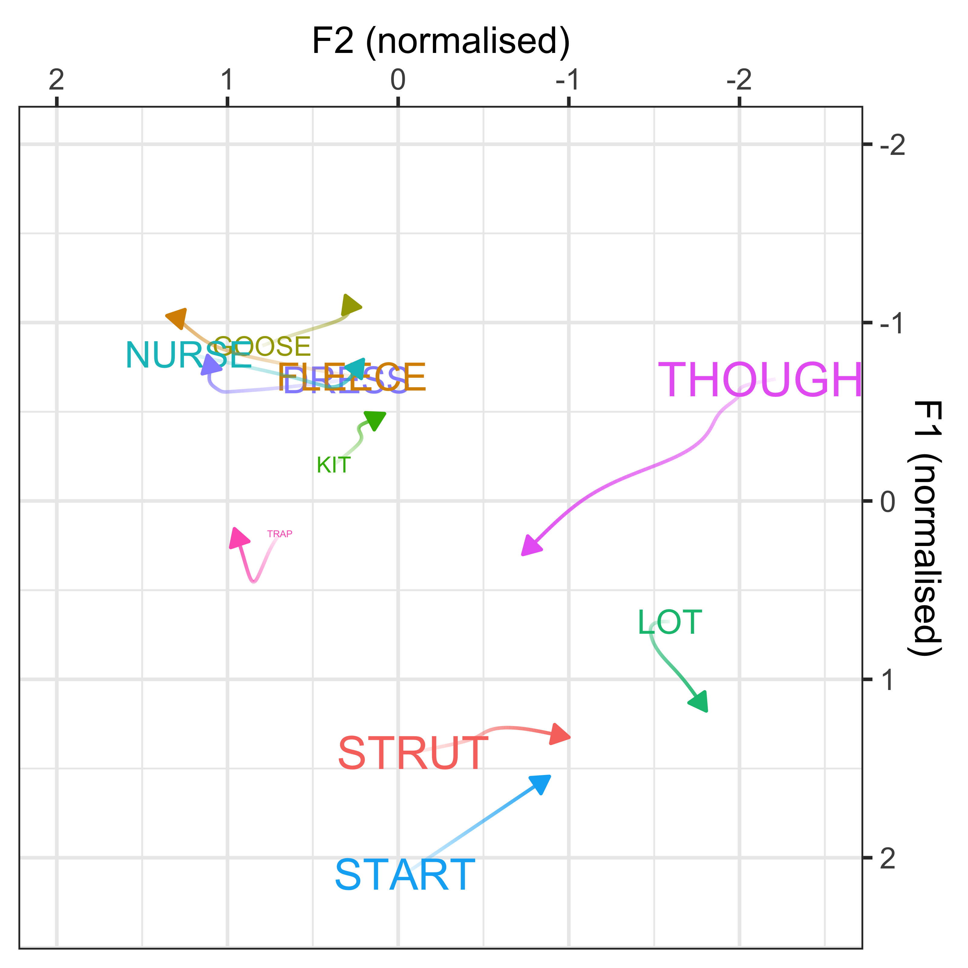

# ggsave(plot = PC1_change_plot, filename = "Figures/PC1_plot_static.png", width = 5.5, height = 5.5, dpi = 300)

Visualisation by animation

• x axis = F2

• y axis = F1

• colours = lexical set of vowel

• movement = trajectory of the F1/F2 in terms PCA score

• trails = the previous positions of the vowels

PC1_plot_animation <- PC1_plot_data %>%
  arrange(Comp.1) %>%
  #set general aesthetics
  ggplot(aes(x = F2, y = F1, colour = Vowel, group = Vowel, label = Vowel)) +
  geom_text(aes(size = PC1_loadings_abs, fontface = 2), show.legend = FALSE) +
  # geom_point() +
  geom_path() +
  #label the axes
  xlab("F2 (normalised)") +
  ylab("F1 (normalised)") +
  #reverse the axes to follow conventional vowel plotting
  scale_x_reverse(limits = c(2,-2.8), position = "top") +
  scale_y_reverse(limits = c(2.3,-2), position = "right") +
  #set the colours
  scale_color_manual(values = c("#9590FF", "#D89000", "#A3A500", "#39B600", "#00BF7D",
                                 "#00BFC4", "#00B0F6", "#F8766D", "#E76BF3", "#FF62BC")) +
  #set the label size
  scale_size_continuous(range = c(1,5)) +
  #add a title
  labs(caption = 'PC1 score: {round(frame_along, 2)}') +
  #set the theme
  theme_bw() +
  #make text more visible
  theme(axis.title = element_text(size = 14, face = "bold"),
        axis.text.x = element_text(size = 14, face = "bold"),
        axis.text.y = element_text(size = 14, face = "bold", angle = 270),
        axis.ticks = element_blank(),
        plot.caption = element_text(size = 30, hjust = 0),
        legend.position = "none") +
  #set the variable for the animation transition i.e. the time dimension
  transition_reveal(Comp.1)

animate(PC1_plot_animation, nframes = 200, fps = 5, rewind = FALSE, start_pause = 10, end_pause = 10, duration = 20)

# anim_save("Figures/PC1_animation.gif")

PC1_plot_animation

PC2

GAMM modelling

#loop through the vowels
for (i in levels(factor(vowels_all$Vowel))) {

  #F1 modelling
  cat(paste0("F1_", i, ": ", format(Sys.time(), "%d %B %Y, %r"), " ✅\n"))  #print the vowel the loop is up to for F1, as well as the start time for the model

  #run the mixed-effects model on the vowel, i.e. if i = FLEECE this will model F1 for FLEECE
  gam.F1 <- bam(F1_lobanov_2.0 ~
                  s(Comp.2, k = 10) +
                  s(Speaker, bs="re") +
                  s(Word, bs="re"),
                data=vowels_all %>% filter(Vowel == i),
                discrete=T, nthreads=2)

  #store the model
  assign(paste0("gam_F1_", i), gam.F1)

  #save the model summary
  saveRDS(gam.F1, file = paste0("/Users/james/Documents/GitHub/model_summaries/PC2/gam_F1_", i, ".rds"))

  #F2 modelling
  cat(paste0("F2_", i, ": ", format(Sys.time(), "%d %B %Y, %r"), " ✅\n"))  #print the vowel the loop is up to for F2 , as well as the start time for the model

  #run the mixed-effects model on the vowel, i.e. if i = FLEECE this will model F2 for FLEECE
  gam.F2 <- bam(F2_lobanov_2.0 ~
                  s(Comp.2, k = 10) +
                  s(Speaker, bs="re") +
                  s(Word, bs="re"),
                data=vowels_all %>% filter(Vowel == i),
                discrete=T, nthreads=2)

  #store the model
  assign(paste0("gam_F2_", i), gam.F2)

  #save the model summary
  saveRDS(gam.F2, file = paste0("/Users/james/Documents/GitHub/model_summaries/PC2/gam_F2_", i, ".rds"))

}

Visualisation by GAM smooth

mod_pred_PC2_values <- readRDS("Data/Models/mod_pred_PC2_values.rds")

#get means for each speaker per vowel and formant
PC2_change_summary <- vowels_all %>%
  group_by(Speaker, Comp.2, Vowel) %>%
  dplyr::summarise(n = n(),
                   F1 = mean(F1_lobanov_2.0),
                   F2 = mean(F2_lobanov_2.0),
                   sd_F1 = sd(F1_lobanov_2.0),
                   sd_F2 = sd(F2_lobanov_2.0)) %>%
  ungroup() %>%
  pivot_longer(F1:F2, names_to = "Formant", values_to = "fit")

#plot the gam smooths predicting F1/F2 per vowel and add the per speaker mean values
PC2_plot_smooth <- mod_pred_PC2_values %>%
  mutate(Formant = factor(Formant, levels = c("F2", "F1"))) %>%
  ggplot(aes(x = -Comp.2, y = fit, colour = Formant, fill = Formant)) +
  geom_point(data = PC2_change_summary %>%
  mutate(Formant = factor(Formant, levels = c("F2", "F1"))), size = 0.25, alpha = 0.1) +
  geom_line(size = 1) +
  geom_ribbon(aes(ymin = ll, ymax = ul), alpha = 0.2, colour = NA) +
  scale_x_continuous(breaks = c(-4, 0, 4)) +
  xlab("PC2 score") +
  ylab("Predicted model fit (Lobanov 2.0)") +
  facet_grid(Formant~Vowel) +
  theme_bw() +
  theme(legend.position = "none", axis.text = element_text(size = 12), axis.title = element_text(size = 14, face = "bold"), strip.text = element_text(size = 12, face = "bold"))

PC2_plot_smooth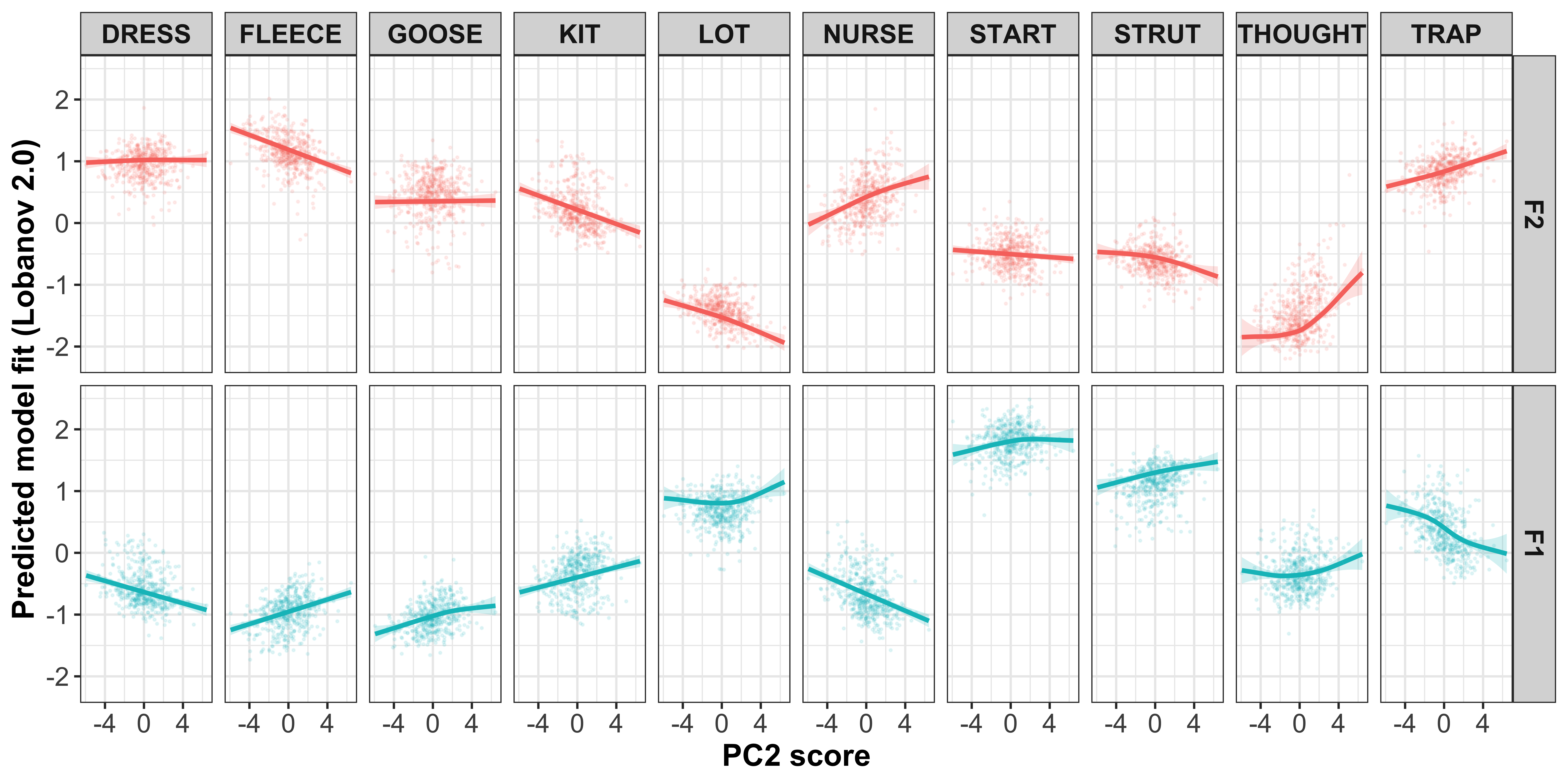

# ggsave(plot = PC2_plot_smooth, filename = "Figures/PC2_plot_gam.png", width = 10, height = 5, dpi = 300)

Visualisation in F1/F2 space

#transform data so there are separate columns for F1 and F2
PC2_plot_data <- mod_pred_PC2_values %>%
  select(Comp.2, fit, Vowel, Formant) %>%
  mutate(Comp.2 = -Comp.2) %>%
  pivot_wider(names_from = Formant, values_from = fit) %>% #transform the data to wide format so there are separate F1 and F2 variables
  left_join(., PC2_loadings %>%
  group_by(Vowel) %>%
  filter(PC2_loadings_abs == max(PC2_loadings_abs)))

#make data frame to plot starting point, this will give the vowel labels based on the smallest PCA scores
PC2_change_labels1 <- PC2_plot_data %>%
  group_by(Vowel) %>%
  filter(Comp.2 == min(Comp.2))

#make data frame to plot end point, this will give the arrow at the end of the paths based on the largest year of birth coordinates
PC2_change_labels2 <- PC2_plot_data %>%
  group_by(Vowel) %>%
  top_n(wt = Comp.2, n = 2)

#plot
PC2_change_plot <- PC2_plot_data %>%
  mutate(PC2_loadings_abs = PC2_loadings_abs) %>%
  #set general aesthetics
  ggplot(aes(x = F2, y = F1, colour = Vowel, alpha = Comp.2, group = Vowel)) +
  #plot the vowel labels
  geom_text(data = PC2_change_labels1, aes(x = F2, y = F1, colour = Vowel, group = Vowel, label = Vowel, size = PC2_loadings_abs), inherit.aes = FALSE, show.legend = FALSE) +
  #add year of birth change trajectories
  geom_path(size = 0.5, show.legend = FALSE) +
  #add end points (this gives the arrows)
  geom_path(data = PC2_change_labels2, aes(x = F2, y = F1, colour = Vowel, group = Vowel),
            arrow = arrow(ends = "first", type = "closed", length = unit(0.2, "cm")),
            inherit.aes = FALSE, show.legend = FALSE) +
  #label the axes
  xlab("F2 (normalised)") +
  ylab("F1 (normalised)") +
  #scale the size so the path is not too wide
  scale_size_continuous(range = c(1,5)) +
  #reverse the axes to follow conventional vowel plotting
  scale_x_reverse(limits = c(2,-2.5), position = "top") +
  scale_y_reverse(limits = c(2.3,-2), position = "right") +
  #set the colours
  scale_color_manual(values = c("#9590FF", "#D89000", "#A3A500", "#39B600", "#00BF7D",
                                 "#00BFC4", "#00B0F6", "#F8766D", "#E76BF3", "#FF62BC")) +
  #add a title
  # labs(title = "B) Change in PC2\n     variance explained = 17.1%") +
  #set the theme
  theme_bw() +
  #make title bold
  theme(plot.title = element_text(face="bold"))

PC2_change_plot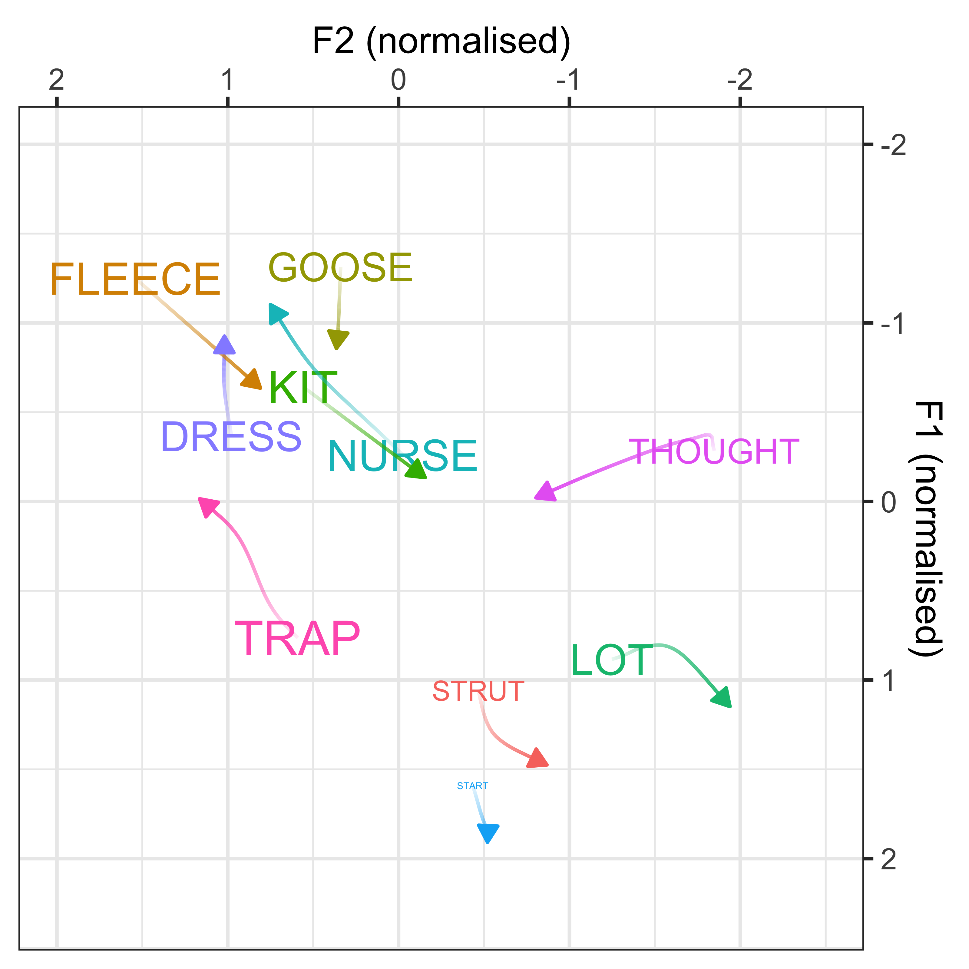

# ggsave(plot = PC2_change_plot, filename = "Figures/PC2_plot_static.png", width = 5.5, height = 5.5, dpi = 300)

Visualisation by animation

PC2_plot_animation <- PC2_plot_data %>%
  arrange(Comp.2) %>%
  #set general aesthetics
  ggplot(aes(x = F2, y = F1, colour = Vowel, group = Vowel, label = Vowel)) +
  geom_text(aes(fontface = 2, size = PC2_loadings_abs), show.legend = FALSE) +
  geom_step() +
  #label the axes
  xlab("F2 (normalised)") +
  ylab("F1 (normalised)") +
  #reverse the axes to follow conventional vowel plotting
  scale_x_reverse(limits = c(2,-2), position = "top") +
  scale_y_reverse(limits = c(2.3,-2), position = "right") +
  #set the colours
  scale_color_manual(values = c("#9590FF", "#D89000", "#A3A500", "#39B600", "#00BF7D",
                                 "#00BFC4", "#00B0F6", "#F8766D", "#E76BF3", "#FF62BC")) +
  #set the label size
  scale_size_continuous(range = c(1,5)) +
  #add a title
  labs(caption = 'PC2 score: {round(frame_along, 2)}') +
  #set the theme
  theme_bw() +
  #make text more visible
  theme(axis.title = element_text(size = 14, face = "bold"),
        axis.text.x = element_text(size = 14, face = "bold"),
        axis.text.y = element_text(size = 14, face = "bold", angle = 270),
        axis.ticks = element_blank(),
        plot.caption = element_text(size = 30, hjust = 0),
        legend.position = "none") +
  #set the variable for the animation transition i.e. the time dimension
  transition_reveal(Comp.2) +
  #add in a trail to see the path
  # shadow_trail(max_frames = 100, alpha = 0.1) +
  ease_aes('linear')

animate(PC2_plot_animation, nframes = 200, fps = 5, rewind = FALSE, start_pause = 10, end_pause = 10, duration = 20)

# anim_save("Figures/PC2_animation.gif")

PC3

GAMM modelling

for (i in levels(factor(vowels_all$Vowel))) {

  #F1 modelling
  cat(paste0("F1_", i, ": ", format(Sys.time(), "%d %B %Y, %r"), " ✅\n"))  #print the vowel the loop is up to for F1, as well as the start time for the model

  #run the mixed-effects model on the vowel, i.e. if i = FLEECE this will model F1 for FLEECE
  gam.F1 <- bam(F1_lobanov_2.0 ~
                  s(Comp.3, k = 10) +
                  s(Speaker, bs="re") +
                  s(Word, bs="re"),
                data=vowels_all %>% filter(Vowel == i),
                discrete=T, nthreads=2)

  #store the model
  assign(paste0("gam_F1_", i), gam.F1)

  #save the model summary
  saveRDS(gam.F1, file = paste0("/Users/james/Documents/GitHub/model_summaries/PC3/gam_F1_", i, ".rds"))

  #F2 modelling
  cat(paste0("F2_", i, ": ", format(Sys.time(), "%d %B %Y, %r"), " ✅\n"))  #print the vowel the loop is up to for F2 , as well as the start time for the model

  #run the mixed-effects model on the vowel, i.e. if i = FLEECE this will model F2 for FLEECE
  gam.F2 <- bam(F2_lobanov_2.0 ~
                  s(Comp.3, k = 10) +
                  s(Speaker, bs="re") +
                  s(Word, bs="re"),
                data=vowels_all %>% filter(Vowel == i),
                discrete=T, nthreads=2)

  #store the model
  assign(paste0("gam_F2_", i), gam.F2)

  #save the model summary
  saveRDS(gam.F2, file = paste0("/Users/james/Documents/GitHub/model_summaries/PC3/gam_F2_", i, ".rds"))

}

Visualisation by GAM smooth

mod_pred_PC3_values <-  readRDS("Data/Models/mod_pred_PC3_values.rds")

#get means for each speaker per vowel and formant
PC3_change_summary <- vowels_all %>%
  group_by(Speaker, Comp.3, Vowel) %>%
  dplyr::summarise(n = n(),
                   F1 = mean(F1_lobanov_2.0),
                   F2 = mean(F2_lobanov_2.0),
                   sd_F1 = sd(F1_lobanov_2.0),
                   sd_F2 = sd(F2_lobanov_2.0)) %>%
  ungroup() %>%
  pivot_longer(F1:F2, names_to = "Formant", values_to = "fit")

#plot the gam smooths predicting F1/F2 per vowel and add the per speaker mean values
PC3_plot_smooth <- mod_pred_PC3_values %>%
  mutate(Formant = factor(Formant, levels = c("F2", "F1"))) %>%
  ggplot(aes(x = -Comp.3, y = fit, colour = Formant, fill = Formant)) +
  geom_point(data = PC3_change_summary %>%
  mutate(Formant = factor(Formant, levels = c("F2", "F1"))), size = 0.25, alpha = 0.1) +
  geom_line(size = 1) +
  geom_ribbon(aes(ymin = ll, ymax = ul), alpha = 0.2, colour = NA) +
  scale_x_continuous(breaks = c(-4, 0, 4)) +
  xlab("PC3 score") +
  ylab("Predicted model fit (Lobanov 2.0)") +
  facet_grid(Formant~Vowel) +
  theme_bw() +
  theme(legend.position = "none", axis.text = element_text(size = 12), axis.title = element_text(size = 14, face = "bold"), strip.text = element_text(size = 12, face = "bold"))

PC3_plot_smooth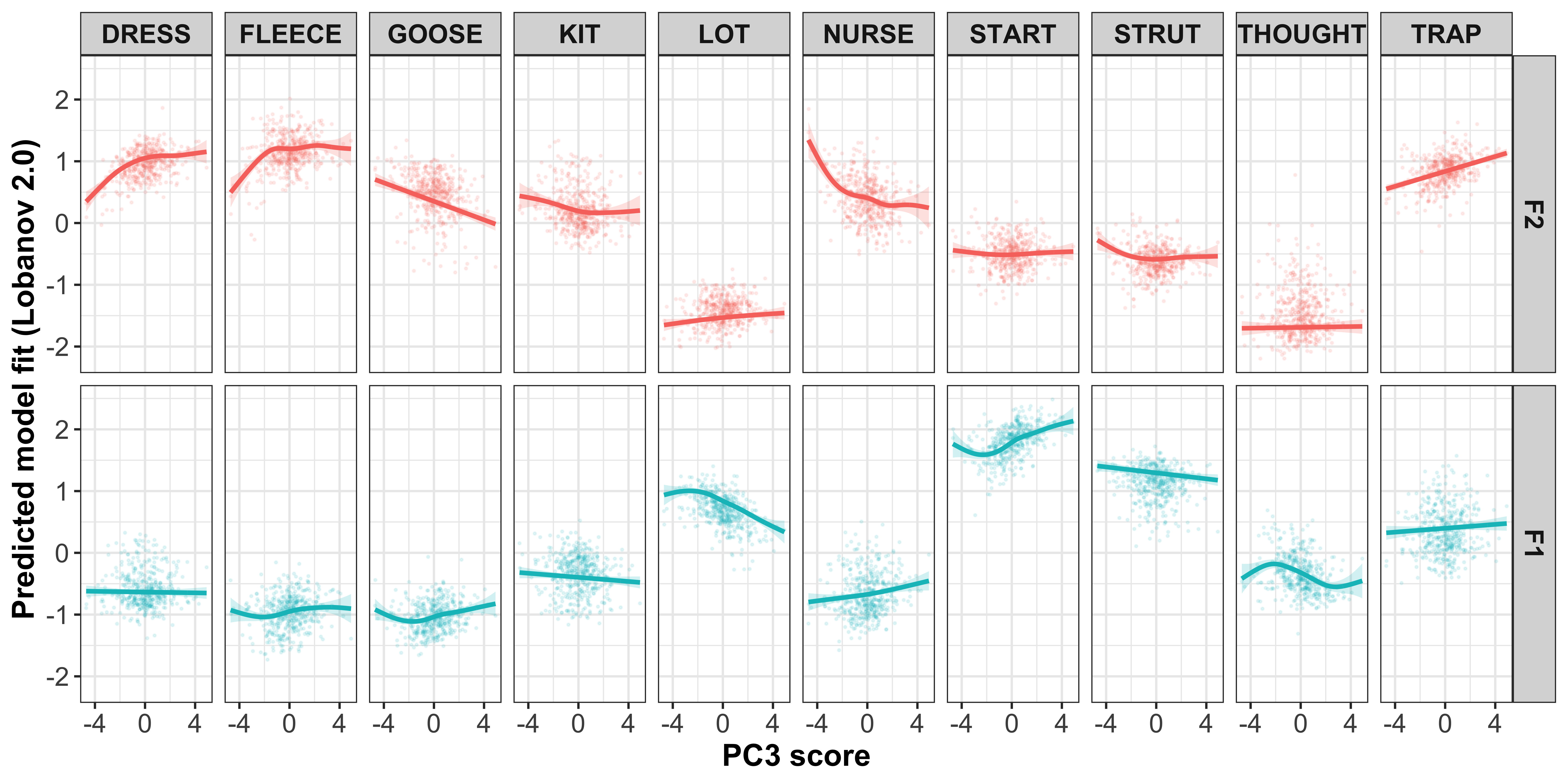

# ggsave(plot = PC3_plot_smooth, filename = "Figures/PC3_plot_gam.png", width = 10, height = 5, dpi = 300)

Visualisation in F1/F2 space

#extract the smoothed values from the plot and store them
#transform data so there are separate columns for F1 and F2
PC3_plot_data <- mod_pred_PC3_values %>%
  select(Comp.3, fit, Vowel, Formant) %>%
  mutate(Comp.3 = -Comp.3) %>%
  pivot_wider(names_from = Formant, values_from = fit) %>% #transform the data to wide format so there are separate F1 and F2 variables
  left_join(., PC3_loadings %>%
  group_by(Vowel) %>%
  filter(PC3_loadings_abs == max(PC3_loadings_abs)))

#make data frame to plot starting point, this will give the vowel labels based on the smallest PCA scores
PC3_change_labels1 <- PC3_plot_data %>%
  group_by(Vowel) %>%
  filter(Comp.3 == min(Comp.3))

#make data frame to plot end point, this will give the arrow at the end of the paths based on the largest year of birth coordinates
PC3_change_labels2 <- PC3_plot_data %>%
  group_by(Vowel) %>%
  top_n(wt = Comp.3, n = 2)

#plot
PC3_change_plot <- PC3_plot_data %>%
  mutate(PC3_loadings_abs = PC3_loadings_abs) %>%
  #set general aesthetics
  ggplot(aes(x = F2, y = F1, colour = Vowel, alpha = Comp.3, group = Vowel)) +
  #plot the vowel labels
  geom_text(data = PC3_change_labels1, aes(x = F2, y = F1, colour = Vowel, group = Vowel, label = Vowel, size = PC3_loadings_abs), inherit.aes = FALSE, show.legend = FALSE) +
  #add year of birth change trajectories
  geom_path(size = 0.5, show.legend = FALSE) +
  #add end points (this gives the arrows)
  geom_path(data = PC3_change_labels2, aes(x = F2, y = F1, colour = Vowel, group = Vowel),
            arrow = arrow(ends = "first", type = "closed", length = unit(0.2, "cm")),
            inherit.aes = FALSE, show.legend = FALSE) +
  #label the axes
  xlab("F2 (normalised)") +
  ylab("F1 (normalised)") +
  #scale the size so the path is not too wide
  scale_size_continuous(range = c(1,5)) +
  #reverse the axes to follow conventional vowel plotting
  scale_x_reverse(limits = c(2,-2.5), position = "top") +
  scale_y_reverse(limits = c(2.3,-2), position = "right") +
  #set the colours
  scale_color_manual(values = c("#9590FF", "#D89000", "#A3A500", "#39B600", "#00BF7D",
                                 "#00BFC4", "#00B0F6", "#F8766D", "#E76BF3", "#FF62BC")) +
  #add a title
  # labs(title = "B) Change in PC3\n     variance explained = 17.1%") +
  #set the theme
  theme_bw() +
  #make title bold
  theme(plot.title = element_text(face="bold"))

PC3_change_plot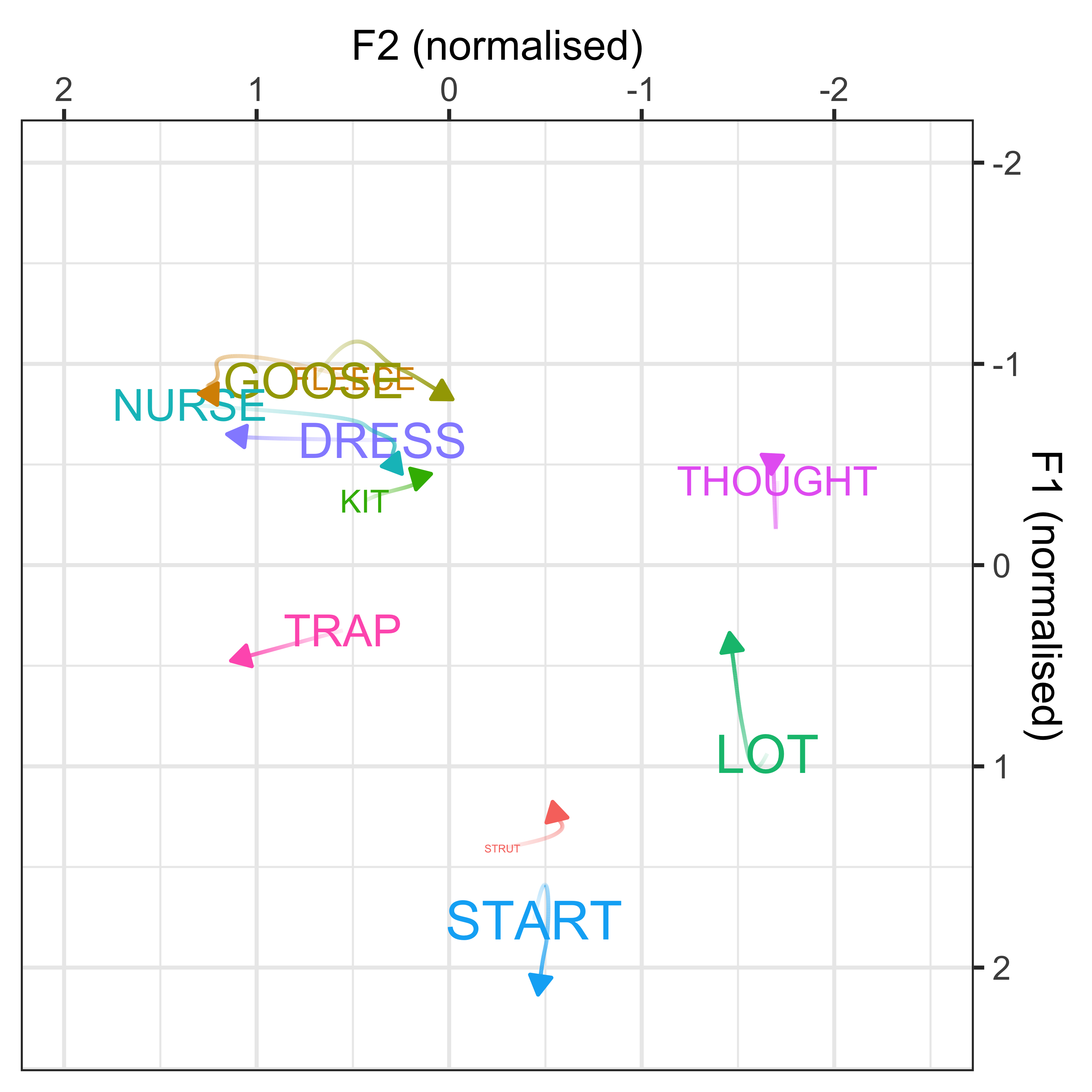

# ggsave(plot = PC3_change_plot, filename = "Figures/PC3_plot_static.png", width = 5.5, height = 5.5, dpi = 300)

Visualisation by animation

PC3_plot_animation <- PC3_plot_data %>%
  arrange(Comp.3) %>%
  #set general aesthetics
  ggplot(aes(x = F2, y = F1, colour = Vowel, group = Vowel, label = Vowel)) +
  geom_text(aes(fontface = 2, size = PC3_loadings_abs), show.legend = FALSE) +
  geom_path() +
  #label the axes
  xlab("F2 (normalised)") +
  ylab("F1 (normalised)") +
  #reverse the axes to follow conventional vowel plotting
  scale_x_reverse(limits = c(2,-2), position = "top") +
  scale_y_reverse(limits = c(2.3,-2), position = "right") +
  #set the colours
  scale_color_manual(values = c("#9590FF", "#D89000", "#A3A500", "#39B600", "#00BF7D",
                                 "#00BFC4", "#00B0F6", "#F8766D", "#E76BF3", "#FF62BC")) +
  #set the label size
  scale_size_continuous(range = c(1,5)) +
  #add a title
  labs(caption = 'PC3 score: {round(frame_along, 2)}') +
  #set the theme
  theme_bw() +
  #make text more visible
  theme(axis.title = element_text(size = 14, face = "bold"),
        axis.text.x = element_text(size = 14, face = "bold"),
        axis.text.y = element_text(size = 14, face = "bold", angle = 270),
        axis.ticks = element_blank(),
        plot.caption = element_text(size = 30, hjust = 0),
        legend.position = "none") +
  #set the variable for the animation transition i.e. the time dimension
  transition_reveal(Comp.3) +
  #add in a trail to see the path
  # shadow_trail(max_frames = 100, alpha = 0.1) +
  ease_aes('linear')

animate(PC3_plot_animation, nframes = 200, fps = 5, rewind = FALSE, start_pause = 10, end_pause = 10, duration = 20)

# anim_save("Figures/PC3_animation.gif")

Comparison with sound change

We can also compare the smooths for the key variables (i.e. contributing > 50% variation) for each PC to the sound change smooths. These plots will use the GAMMs predicting F1/F2 by the PCA scores again,

To do this, we first select the key variables for each PC, filtering the data so only those key variables are visualised.

We then need to take the smooths from the initial GAMMs (i.e. those used to extract the speaker intercepts).

Note, it is important to scale the year_of_birth variable from these models so a comparison can be made with the PC scores. This is done by scaling to a range based on the PC scores, so the earliest year of birth represents the smallest score, whereas the most recent year of birth represents the highest score. This preseves the data and the smooths can be compared, but it simply makes visualisation easier.

PC1

#select the key vairables from the PCA
mod_pred_PC1_values1 <- mod_pred_PC1_values %>%
  select(Comp.1, fit, ul, ll, Vowel, Formant) %>%
  mutate(Comp.1 = -Comp.1,
         Variable = paste0(Formant, "_", Vowel),
         var = "PC1",
         participant_year_of_birth = rescale(Comp.1, to = range(mod_pred_PC1_values$participant_year_of_birth))) #rescale the year of birth variable

PC1_contrib <- PC1_contrib %>%
  mutate(Formant = substr(Variable, 1, 2),
         x = ifelse(Formant == "F1", -3.2, 2.8),
         y = -2.75,
         x1 = ifelse(Vowel != "THOUGHT", (min(mod_pred_PC1_values1$Comp.1)+max(mod_pred_PC1_values1$Comp.1))/2, x)) %>%
  group_by(Vowel) %>%
  mutate(Contribution.PC1_max = max(Contribution.PC1)) %>%
  ungroup() %>%
  mutate(Vowel = factor(.$Vowel, levels=unique(.$Vowel[order(.$Contribution.PC1_max)]), ordered=TRUE)) %>%
  group_by(Vowel)

#match the data to the year of birth smooths
mod_pred_yob_values1 <- mod_pred_yob_values %>%
  select(participant_year_of_birth, fit, ul, ll, Vowel, Formant) %>%
  mutate(Variable = paste0(Formant, "_", Vowel),
         var = "yob",
         #rescale the year of birth variable
         Comp.1 = rescale(participant_year_of_birth, to = range(mod_pred_PC1_values1$Comp.1))) %>%
  filter(Variable %in% mod_pred_PC1_values1$Variable) %>%
  rbind(mod_pred_PC1_values1) %>% #combine with the PCA scores data
  left_join(., PC1_contrib %>% select(Variable, Contribution.PC1)) %>% #get contribution values
  mutate(Contribution.PC1a = paste0(round(Contribution.PC1, 1), "%")) %>%
  #reorder the Vowel factor so it is ordered by contribution
  group_by(Vowel) %>%
  mutate(Contribution.PC1_max = max(Contribution.PC1)) %>%
  ungroup() %>%
  mutate(Vowel = factor(.$Vowel, levels=unique(.$Vowel[order(.$Contribution.PC1_max)]), ordered=TRUE)) %>%
  left_join(PC1_contrib %>% select(Variable, cumsum_PC1, highlight))

#plot all model smooths facetted by vowel
PC1_plot_smooth1 <- mod_pred_yob_values1 %>%
  mutate(Formant = factor(Formant, levels = c("F2", "F1"))) %>%
  ggplot(aes(x = Comp.1, y = fit, colour = Formant, fill = Formant, linetype = var)) +
  geom_line() + #smooth line
  geom_ribbon(aes(ymin = ll, ymax = ul), alpha = 0.1, colour = NA) + #confidence intervals
  scale_x_continuous(breaks = c(-4, 0, 4),
                     sec.axis = dup_axis(breaks = c(-2.80243, 2.071311), labels = c(1900, 1950), name = "Participant year of birth"),  #add secondary axis for year of birth, this is done by rescaling the loading values to scale of year of birth
                     name = "PC1 score"
                     ) +
  scale_y_reverse(breaks = seq(-2, 2, 1), limits = c(2.5, -2.9)) + #revese the axis so it follows convention
  scale_linetype(name = NULL) + #remove the name (var) from the legend
  ylab("Predicted model fit (Lobanov 2.0)") +
  facet_grid(Formant~Vowel) +
  geom_label(data = PC1_contrib %>%
  mutate(Formant = factor(Formant, levels = c("F2", "F1"))), aes(x = 0, y = y, label = paste0(round(Contribution.PC1, 1), "%"), colour = Formant), size = 3, inherit.aes = FALSE, show.legend = FALSE) +
  theme_bw()  +
  theme(legend.position = "top", axis.text = element_text(size = 12), axis.title = element_text(size = 14, face = "bold"), strip.text = element_text(size = 12, face = "bold")) +
  guides(linetype=guide_legend(override.aes=list(fill=NA)))

PC1_plot_smooth1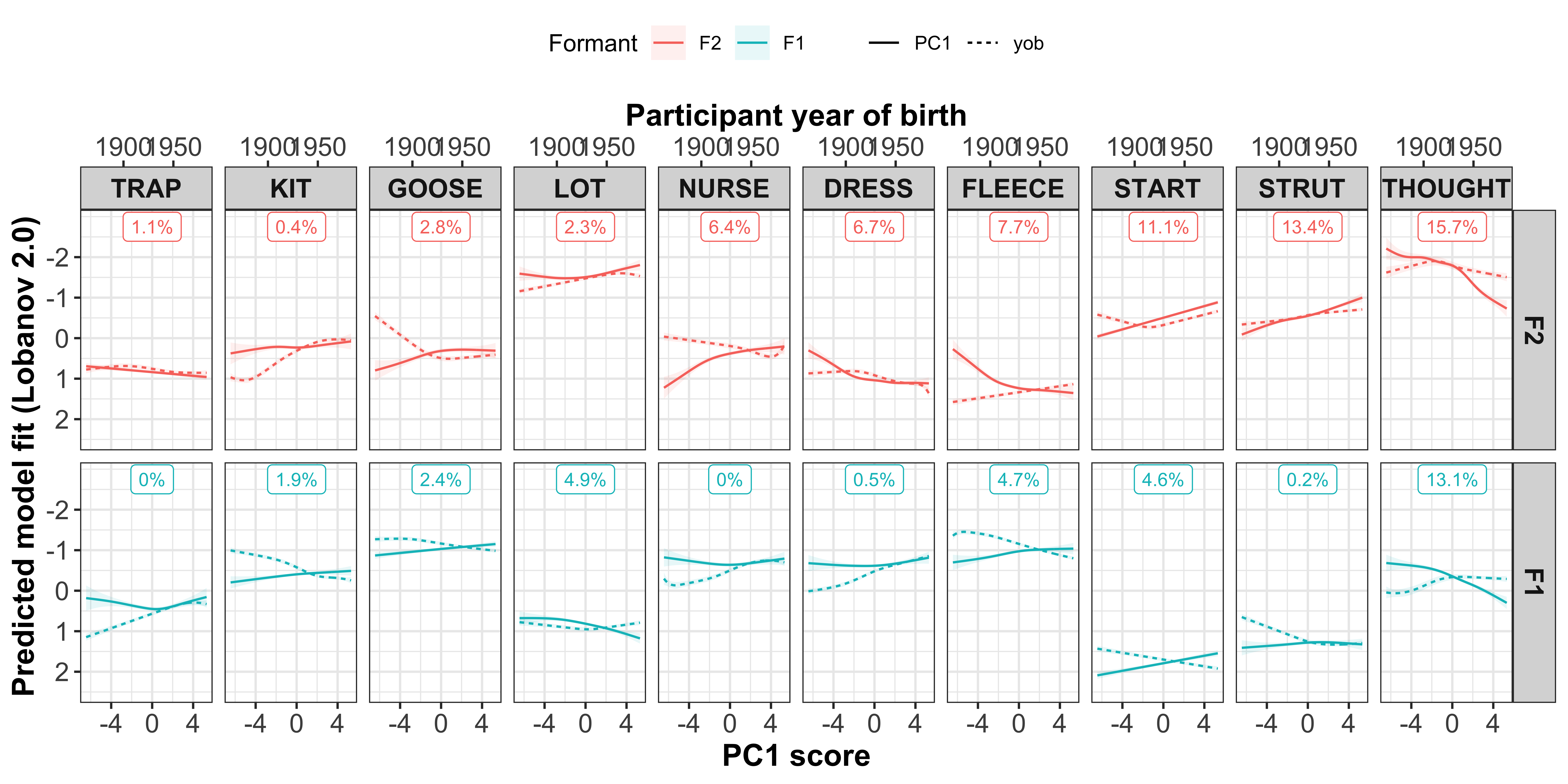

# ggsave(plot = PC1_plot_smooth1, filename = "Figures/PC1_yob.png", width = 11, height = 5, dpi = 300)

#plot all model smooths facetted by vowel
PC1_plot_smooth_important <- mod_pred_yob_values1 %>%
  filter(highlight == "black") %>%
  mutate(Vowel = ifelse(Vowel == "THOUGHT", paste0(Vowel, " (", Formant, ")"), as.character(Vowel))) %>%
  ggplot(aes(x = Comp.1, y = fit, colour = Formant, fill = Formant, linetype = var)) +
  geom_line() + #smooth line
  geom_ribbon(aes(ymin = ll, ymax = ul), alpha = 0.1, colour = NA) + #confidence intervals
  scale_x_continuous(breaks = c(-4, 0, 4),
                     sec.axis = dup_axis(breaks = c(-2.80243, 2.071311), labels = c(1900, 1950), name = "Participant year of birth"),  #add secondary axis for year of birth, this is done by rescaling the loading values to scale of year of birth
                     name = "PC1 score"
                     ) +
  scale_y_reverse(breaks = seq(-2, 2, 1), limits = c(2.5, -2.9)) + #revese the axis so it follows convention
  scale_linetype(name = NULL) + #remove the name (var) from the legend
  ylab("Predicted model fit (Lobanov 2.0)") +
  facet_grid(~Vowel) +
  geom_label(data = PC1_contrib %>% ungroup() %>% filter(highlight == "black") %>%
  mutate(Vowel = ifelse(Vowel == "THOUGHT", paste0(Vowel, " (", Formant, ")"), as.character(Vowel))), aes(x = 0, y = y, label = paste0(round(Contribution.PC1, 1), "%"), colour = Formant), size = 3, inherit.aes = FALSE, show.legend = FALSE) +
  theme_bw() +
  theme(axis.text = element_text(size = 12), axis.title = element_text(size = 14, face = "bold"), strip.text = element_text(size = 12, face = "bold")) +
  guides(linetype=guide_legend(override.aes=list(fill=NA)))

PC1_plot_smooth_important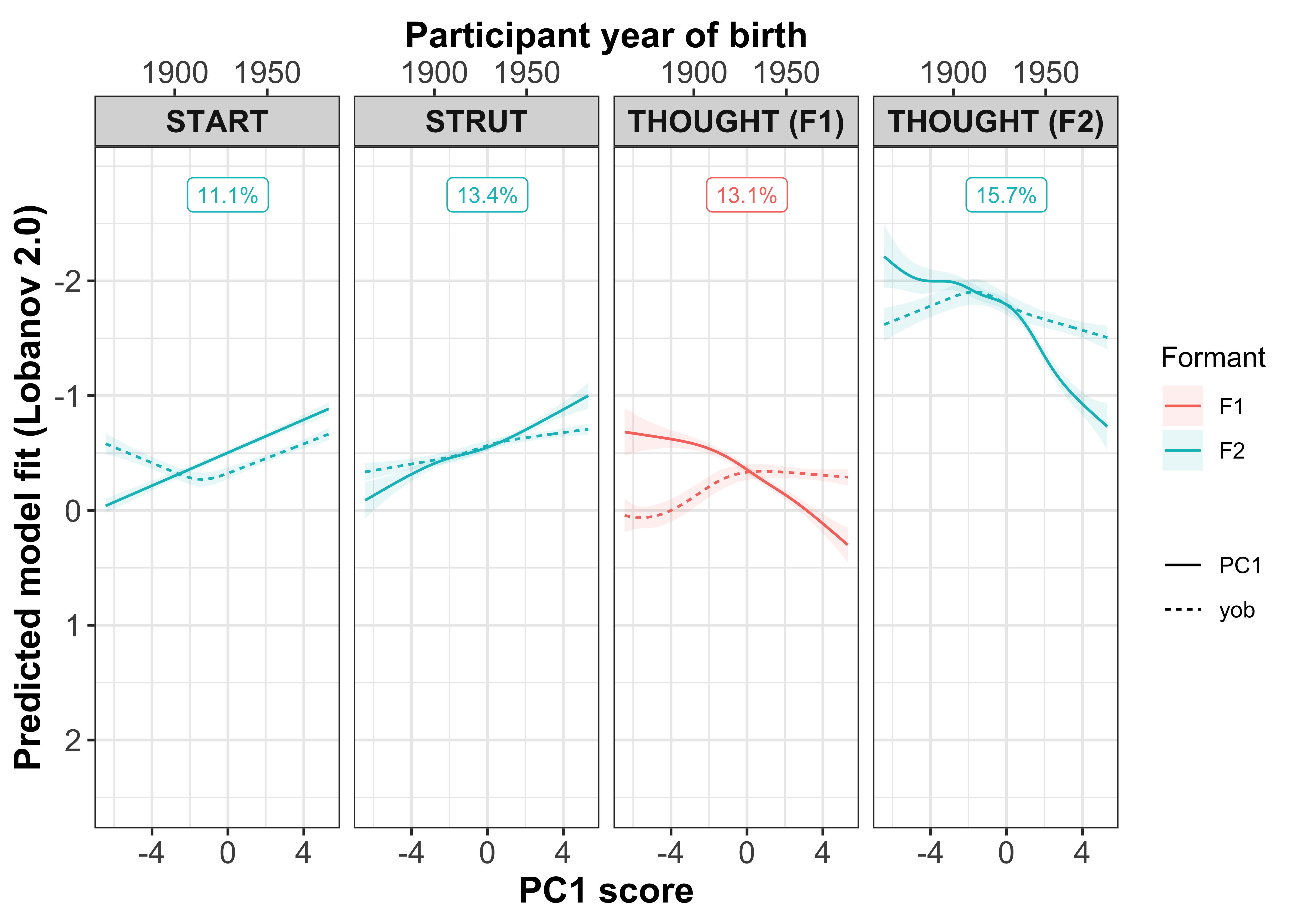

# ggsave(plot = PC1_plot_smooth_important, filename = "Figures/PC1_yob_important.png", width = 5, height = 5, dpi = 300)

PC2

mod_pred_PC2_values2 <- mod_pred_PC2_values %>%
  select(Comp.2, fit, ul, ll, Vowel, Formant) %>%
  mutate(Comp.2 = -Comp.2,
         Variable = paste0(Formant, "_", Vowel),
         var = "PC2",
         participant_year_of_birth = rescale(Comp.2, to = range(mod_pred_yob_values$participant_year_of_birth)))

PC2_contrib <- PC2_contrib %>%
  mutate(Formant = substr(Variable, 1, 2),
         x = ifelse(Formant == "F1", -3, 3),
         y = -2.75) %>%
  group_by(Vowel) %>%
  mutate(Contribution.PC2_max = max(Contribution.PC2)) %>%
  ungroup() %>%
  mutate(Vowel = factor(.$Vowel, levels=unique(.$Vowel[order(.$Contribution.PC2_max)]), ordered=TRUE)) %>%
  group_by(Vowel)

mod_pred_yob_values2 <- mod_pred_yob_values %>%
  select(participant_year_of_birth, fit, ul, ll, Vowel, Formant) %>%
  mutate(Variable = paste0(Formant, "_", Vowel),
         var = "yob",
         Comp.2 = rescale(participant_year_of_birth, to = range(mod_pred_PC2_values2$Comp.2))) %>%
  filter(Variable %in% mod_pred_PC2_values2$Variable) %>%
  rbind(mod_pred_PC2_values2) %>%
  left_join(., PC2_contrib %>% select(Variable, Contribution.PC2)) %>%
  mutate(Contribution.PC2a = paste0(round(Contribution.PC2, 1), "%")) %>%
  group_by(Vowel) %>%
  mutate(Contribution.PC2_max = max(Contribution.PC2)) %>%
  ungroup() %>%
  mutate(Vowel = factor(.$Vowel, levels=unique(.$Vowel[order(.$Contribution.PC2_max)]), ordered=TRUE)) %>%
  left_join(PC2_contrib %>% select(Variable, cumsum_PC2, highlight))

#plot all model smooths facetted by vowel
PC2_plot_smooth1 <- mod_pred_yob_values2 %>%
  mutate(Formant = factor(Formant, levels = c("F2", "F1"))) %>%
  ggplot(aes(x = Comp.2, y = fit, colour = Formant, fill = Formant, linetype = var)) +
  geom_line() +
  geom_ribbon(aes(ymin = ll, ymax = ul), alpha = 0.1, colour = NA) +
  scale_x_continuous(breaks = c(-4, 0, 4),
                     sec.axis = dup_axis(breaks = c(-2.103943, 3.018724), labels = c(1900, 1950), name = "Participant year of birth"),  #add secondary axis for year of birth, this is done by rescaling the loading values to scale of year of birth
                     name = "PC2 score"
                     ) +
  scale_y_reverse(breaks = seq(-2, 2, 1), limits = c(2.5, -2.9)) +
  ylab("Predicted model fit (Lobanov 2.0)") +
  scale_linetype(name = NULL) +
  facet_grid(Formant~Vowel) +
  geom_label(data = PC2_contrib %>%
  mutate(Formant = factor(Formant, levels = c("F2", "F1"))), aes(x = 0, y = y, label = paste0(round(Contribution.PC2, 1), "%"), colour = Formant), size = 3, inherit.aes = FALSE, show.legend = FALSE) +
  theme_bw() +
  theme(axis.text = element_text(size = 12), axis.title = element_text(size = 14, face = "bold"), strip.text = element_text(size = 12, face = "bold")) +
  guides(linetype=guide_legend(override.aes=list(fill=NA)))

PC2_plot_smooth1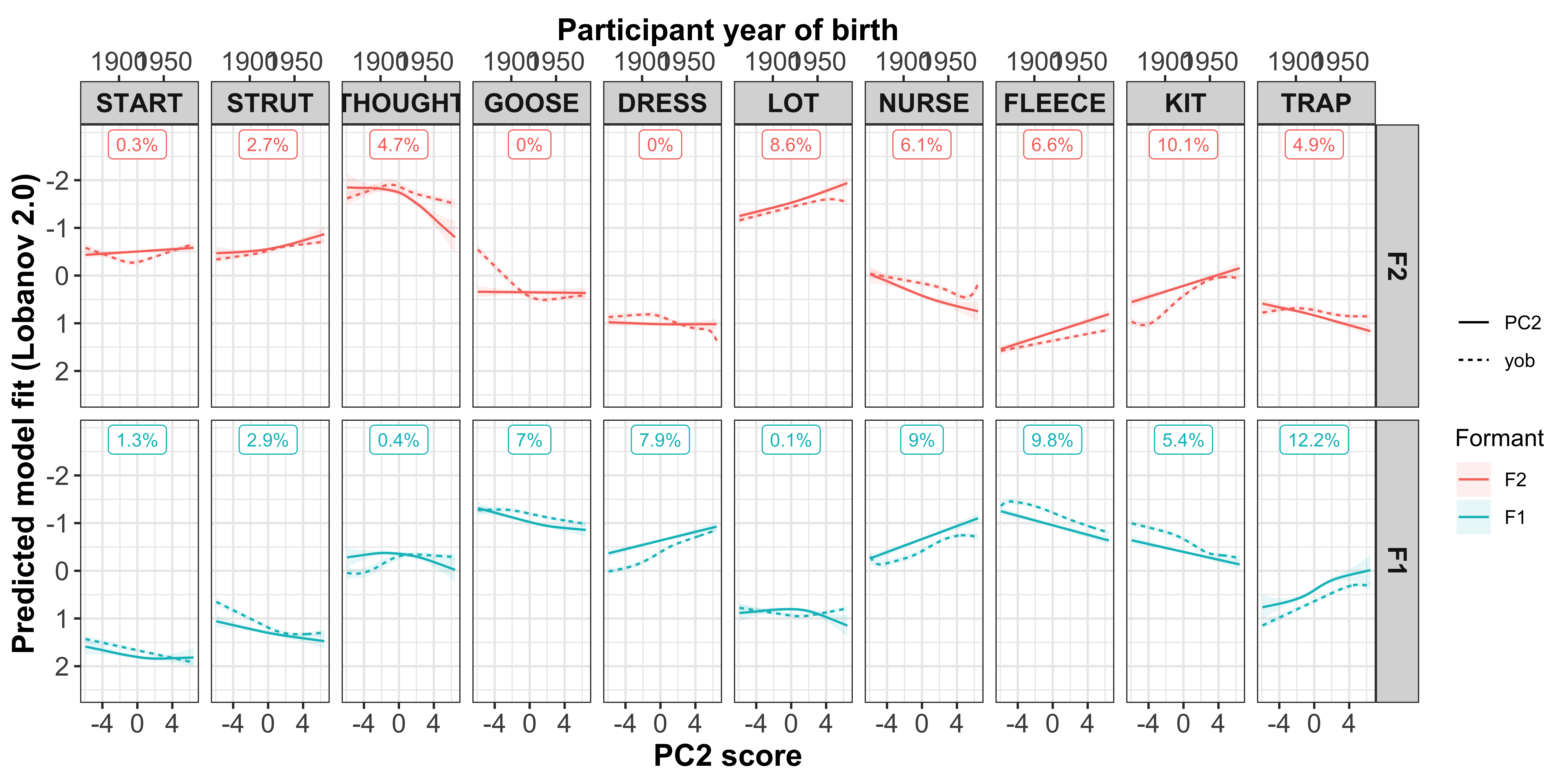

# ggsave(plot = PC2_plot_smooth1, filename = "Figures/PC2_yob.png", width = 11, height = 5)

#plot all model smooths facetted by vowel
PC2_plot_smooth1_important <- mod_pred_yob_values2 %>%
  filter(highlight == "black") %>%
  ggplot(aes(x = Comp.2, y = fit, colour = Formant, fill = Formant, linetype = var)) +
  geom_line() +
  geom_ribbon(aes(ymin = ll, ymax = ul), alpha = 0.1, colour = NA) +
  scale_x_continuous(breaks = c(-4, 0, 4),
                     sec.axis = dup_axis(breaks = c(-2.103943, 3.018724), labels = c(1900, 1950), name = "Participant year of birth"),  #add secondary axis for year of birth, this is done by rescaling the loading values to scale of year of birth
                     name = "PC2 score"
                     ) +
  scale_y_reverse(breaks = seq(-2, 2, 1), limits = c(2.5, -2.9)) +
  ylab("Predicted model fit (Lobanov 2.0)") +
  scale_linetype(name = NULL) +
  facet_grid(~Vowel) +
  geom_label(data = PC2_contrib %>% filter(highlight == "black"), aes(x = 0, y = y, label = paste0(round(Contribution.PC2, 1), "%"), colour = Formant), size = 3, inherit.aes = FALSE, show.legend = FALSE) +
  theme_bw() +
  theme(axis.text = element_text(size = 12), axis.title = element_text(size = 14, face = "bold"), strip.text = element_text(size = 12, face = "bold")) +
  guides(linetype=guide_legend(override.aes=list(fill=NA)))

PC2_plot_smooth1_important

# ggsave(plot = PC2_plot_smooth1_important, filename = "Figures/PC2_yob_important.png", width = 7, height = 5)

PC3

mod_pred_PC3_values3 <- mod_pred_PC3_values %>%
  select(Comp.3, fit, ul, ll, Vowel, Formant) %>%
  mutate(Comp.3 = -Comp.3,
         Variable = paste0(Formant, "_", Vowel),
         var = "PC3",
         participant_year_of_birth = rescale(Comp.3, to = range(mod_pred_yob_values$participant_year_of_birth)))

PC3_contrib <- PC3_contrib %>%
  mutate(Formant = substr(Variable, 1, 2),
         x = ifelse(Formant == "F1", -2.7, 2.7),
         y = -2.75) %>%
  group_by(Vowel) %>%
  mutate(Contribution.PC3_max = max(Contribution.PC3)) %>%
  ungroup() %>%
  mutate(Vowel = factor(.$Vowel, levels=unique(.$Vowel[order(.$Contribution.PC3_max)]), ordered=TRUE)) %>%
  group_by(Vowel)

mod_pred_yob_values3 <- mod_pred_yob_values %>%
  select(participant_year_of_birth, fit, ul, ll, Vowel, Formant) %>%
  mutate(Variable = paste0(Formant, "_", Vowel),
         var = "yob",
         Comp.3 = rescale(participant_year_of_birth, to = range(mod_pred_PC3_values3$Comp.3))) %>%
  filter(Variable %in% mod_pred_PC3_values3$Variable) %>%
  rbind(mod_pred_PC3_values3) %>%
  left_join(., PC3_contrib %>% select(Variable, Contribution.PC3)) %>%
  mutate(Contribution.PC3a = paste0(round(Contribution.PC3, 1), "%"),
         colour1 = ifelse(grepl("F1", Variable), "#F8766D", "#00BFC4")) %>%
  group_by(Vowel) %>%
  mutate(Contribution.PC3_max = max(Contribution.PC3)) %>%
  ungroup() %>%
  mutate(Vowel = factor(.$Vowel, levels=unique(.$Vowel[order(.$Contribution.PC3_max)]), ordered=TRUE)) %>%
  left_join(PC3_contrib %>% select(Variable, cumsum_PC3, highlight))

#plot all model smooths facetted by vowel
PC3_plot_smooth1 <- mod_pred_yob_values3 %>%
  mutate(Formant = factor(Formant, levels = c("F2", "F1"))) %>%
  ggplot(aes(x = Comp.3, y = fit, colour = Formant, fill = Formant, linetype = var)) +
  geom_line() +
  geom_ribbon(aes(ymin = ll, ymax = ul), alpha = 0.1, colour = NA) +
  scale_x_continuous(breaks = c(-4, 0, 4),
                     limits = c(-5, 5),
                     sec.axis = dup_axis(breaks = c(-1.71819, 2.261738), labels = c(1900, 1950), name = "Participant year of birth"),  #add secondary axis for year of birth, this is done by rescaling the loading values to scale of year of birth
                     name = "PC3 score"
                     ) +
  scale_y_reverse(breaks = seq(-2, 2, 1), limits = c(2.5, -2.9)) + #revese the axis so it follows convention
  scale_linetype(name = NULL) +
  xlab("PC3 score") +
  facet_grid(Formant~Vowel) +
  geom_label(data = PC3_contrib %>%
  mutate(Formant = factor(Formant, levels = c("F2", "F1"))), aes(x = 0, y = y, label = paste0(round(Contribution.PC3, 1), "%"), colour = Formant), size = 3, inherit.aes = FALSE, show.legend = FALSE) +
  theme_bw() +
  theme(legend.position = "top", axis.text = element_text(size = 12), axis.title = element_text(size = 14, face = "bold"), strip.text = element_text(size = 12, face = "bold")) +
  guides(linetype=guide_legend(override.aes=list(fill=NA)))

PC3_plot_smooth1

# ggsave(plot = PC3_plot_smooth1, filename = "Figures/PC3_yob.png", width = 11, height = 5)

#plot all model smooths facetted by vowel
PC3_plot_smooth1_important <- mod_pred_yob_values3 %>%
  filter(highlight == "black") %>%
  ggplot(aes(x = Comp.3, y = fit, colour = Formant, fill = Formant, linetype = var)) +
  geom_line() +
  geom_ribbon(aes(ymin = ll, ymax = ul), alpha = 0.1, colour = NA) +
  scale_x_continuous(breaks = c(-4, 0, 4),
                     limits = c(-5, 5),
                     sec.axis = dup_axis(breaks = c(-1.71819, 2.261738), labels = c(1900, 1950), name = "Participant year of birth"),  #add secondary axis for year of birth, this is done by rescaling the loading values to scale of year of birth
                     name = "PC3 score"
                     ) +
  scale_y_reverse(breaks = seq(-2, 2, 1), limits = c(2.5, -2.9)) + #revese the axis so it follows convention
  scale_linetype(name = NULL) +
  xlab("PC3 score") +
  facet_grid(~Vowel) +
  geom_label(data = PC3_contrib %>% filter(highlight == "black"), aes(x = 0, y = y, label = paste0(round(Contribution.PC3, 1), "%"), colour = Formant), size = 3, inherit.aes = FALSE, show.legend = FALSE) +
  theme_bw() +
  theme(axis.text = element_text(size = 12), axis.title = element_text(size = 14, face = "bold"), strip.text = element_text(size = 12, face = "bold")) +
  guides(linetype=guide_legend(override.aes=list(fill=NA)))

PC3_plot_smooth1_important

# ggsave(plot = PC3_plot_smooth1_important, filename = "Figures/PC3_yob_important.png", width = 6, height = 5)

Combined

To inspect the variables easily in one plot, we will now put the sound change plots and the PC plots together.

vowel_plots_combined <- plot_grid(sound_change_plot, PC1_change_plot, PC2_change_plot, PC3_change_plot, nrow = 1)

vowel_plots_combined1 <- plot_grid(NULL, NULL, NULL, NULL, nrow = 1, labels=c("A) Sound change", "B) PC1: var = 17.2%", "C) PC2: var = 15.8%", "D) PC3: var = 10.1%"), hjust = 0, label_size = 20)

vowel_plots_combined <- plot_grid(vowel_plots_combined1, vowel_plots_combined, nrow = 2, rel_heights = c(0.07, 1))

vowel_plots_combined

# ggsave(plot = vowel_plots_combined, filename = "Figures/vowel_plots_combined.png", width = 20, height = 6, dpi = 300)

Example speakers

To get an idea of how the vowel spaces of the speakers on the margins differ, i.e. those with the largest absolute PC socres, we can inspect the 12 speakers who have either the largest/smallest PC scores.

First, we will filter the data to focus on these 24 speakers.

PC_example_test <- vowels_all %>%
  group_by(Speaker, participant_year_of_birth, Gender, Vowel) %>%
  dplyr::summarise(F1_mean = mean(F1_lobanov_2.0),
            F2_mean = mean(F2_lobanov_2.0)) %>%
  left_join(PC_speaker_loadings %>% select(Speaker, Comp.1:Comp.3)) %>%
  left_join(PC1_change_labels1 %>% select(Vowel, PC1_loadings_abs)) %>%
  left_join(PC2_change_labels1 %>% select(Vowel, PC2_loadings_abs)) %>%
  left_join(PC3_change_labels1 %>% select(Vowel, PC3_loadings_abs)) %>%
  ungroup() %>%
  mutate(example_speaker = paste0(Speaker, " (", participant_year_of_birth, ")"),
         example1_PC1 = ifelse(dense_rank(Comp.1) <= 12, "high",
                               ifelse(dense_rank(-Comp.1) <= 12, "low", "normal")),
         example1_PC2 = ifelse(dense_rank(Comp.2) <= 12, "high",
                               ifelse(dense_rank(-Comp.2) <= 12, "low", "normal")),
         example1_PC3 = ifelse(dense_rank(Comp.3) <= 12, "high",
                               ifelse(dense_rank(-Comp.3) <= 12, "low", "normal")))

PC1

PC1_example_test_low <- PC_example_test %>%
  filter(example1_PC1 == "low") %>%
  mutate(example_speaker = factor(.$example_speaker, levels=unique(.$example_speaker[order(.$participant_year_of_birth)]), ordered=TRUE)) %>%
  ggplot(aes(x = F2_mean, y = F1_mean, label = Vowel, colour = Vowel)) +
  scale_color_manual(values = c("#9590FF", "#D89000", "#A3A500", "#39B600", "#00BF7D",
                                      "#00BFC4", "#00B0F6", "#F8766D", "#E76BF3", "#FF62BC")) +
  scale_size_continuous(range = c(2,5)) +
  geom_text(aes(size = PC1_loadings_abs), show.legend = FALSE) +
  scale_x_reverse(position = "top", name = "F2 (normalised)", limits = c(2.4, -2.4)) +
        scale_y_reverse(position = "right", name = "F1 (normalised)", limits = c(2.4, -2.4)) +
  theme(plot.title = element_text(size = 20, face = "italic")) +
  facet_wrap(~factor(example_speaker)) +
  theme_bw()

PC1_example_test_high <- PC_example_test %>%
  filter(example1_PC1 == "high") %>%
  mutate(example_speaker = factor(.$example_speaker, levels=unique(.$example_speaker[order(.$participant_year_of_birth)]), ordered=TRUE)) %>%
  ggplot(aes(x = F2_mean, y = F1_mean, label = Vowel, colour = Vowel)) +
  scale_color_manual(values = c("#9590FF", "#D89000", "#A3A500", "#39B600", "#00BF7D",
                                      "#00BFC4", "#00B0F6", "#F8766D", "#E76BF3", "#FF62BC")) +
  scale_size_continuous(range = c(2,5)) +
  geom_text(aes(size = PC1_loadings_abs), show.legend = FALSE) +
  scale_x_reverse(position = "top", name = "F2 (normalised)", limits = c(2.4, -2.4)) +
        scale_y_reverse(position = "right", name = "F1 (normalised)", limits = c(2.4, -2.4)) +
  theme(plot.title = element_text(size = 20, face = "italic")) +
  facet_wrap(~factor(example_speaker)) +
  theme_bw()

# ggsave(plot = PC1_example_test_low, filename = "Figures/PC1_examples_low.png", width = 15, height = 15, dpi = 300)
# 
# ggsave(plot = PC1_example_test_high, filename = "Figures/PC1_examples_high.png", width = 15, height = 15, dpi = 300)

PC1_example_test_high

PC1_example_test_low

PC2

PC2_example_test_low <- PC_example_test %>%
  filter(example1_PC2 == "low") %>%
  mutate(example_speaker = factor(.$example_speaker, levels=unique(.$example_speaker[order(.$participant_year_of_birth)]), ordered=TRUE)) %>%
  ggplot(aes(x = F2_mean, y = F1_mean, label = Vowel, colour = Vowel)) +
  scale_color_manual(values = c("#9590FF", "#D89000", "#A3A500", "#39B600", "#00BF7D",
                                      "#00BFC4", "#00B0F6", "#F8766D", "#E76BF3", "#FF62BC")) +
  scale_size_continuous(range = c(2,5)) +
  geom_text(aes(size = PC2_loadings_abs), show.legend = FALSE) +
  scale_x_reverse(position = "top", name = "F2 (normalised)", limits = c(2.4, -2.4)) +
        scale_y_reverse(position = "right", name = "F1 (normalised)", limits = c(2.4, -2.4)) +
  theme(plot.title = element_text(size = 20, face = "italic")) +
  facet_wrap(~factor(example_speaker)) +
  theme_bw()

PC2_example_test_high <- PC_example_test %>%
  filter(example1_PC2 == "high") %>%
  mutate(example_speaker = factor(.$example_speaker, levels=unique(.$example_speaker[order(.$participant_year_of_birth)]), ordered=TRUE)) %>%
  ggplot(aes(x = F2_mean, y = F1_mean, label = Vowel, colour = Vowel)) +
  scale_color_manual(values = c("#9590FF", "#D89000", "#A3A500", "#39B600", "#00BF7D",
                                      "#00BFC4", "#00B0F6", "#F8766D", "#E76BF3", "#FF62BC")) +
  scale_size_continuous(range = c(2,5)) +
  geom_text(aes(size = PC2_loadings_abs), show.legend = FALSE) +
  scale_x_reverse(position = "top", name = "F2 (normalised)", limits = c(2.4, -2.4)) +
        scale_y_reverse(position = "right", name = "F1 (normalised)", limits = c(2.4, -2.4)) +
  theme(plot.title = element_text(size = 20, face = "italic")) +
  facet_wrap(~factor(example_speaker)) +
  theme_bw()

# ggsave(plot = PC2_example_test_low, filename = "Figures/PC2_examples_low.png", width = 15, height = 15, dpi = 300)
# 
# ggsave(plot = PC2_example_test_high, filename = "Figures/PC2_examples_high.png", width = 15, height = 15, dpi = 300)

PC2_example_test_high

PC2_example_test_low

PC3

PC3_example_test_low <- PC_example_test %>%
  filter(example1_PC3 == "low") %>%
  mutate(example_speaker = factor(.$example_speaker, levels=unique(.$example_speaker[order(.$participant_year_of_birth)]), ordered=TRUE)) %>%
  ggplot(aes(x = F2_mean, y = F1_mean, label = Vowel, colour = Vowel)) +
  scale_color_manual(values = c("#9590FF", "#D89000", "#A3A500", "#39B600", "#00BF7D",
                                      "#00BFC4", "#00B0F6", "#F8766D", "#E76BF3", "#FF62BC")) +
  scale_size_continuous(range = c(2,5)) +
  geom_text(aes(size = PC3_loadings_abs), show.legend = FALSE) +
  scale_x_reverse(position = "top", name = "F2 (normalised)", limits = c(2.4, -2.4)) +
        scale_y_reverse(position = "right", name = "F1 (normalised)", limits = c(2.4, -2.4)) +
  theme(plot.title = element_text(size = 20, face = "italic")) +
  facet_wrap(~factor(example_speaker)) +
  theme_bw()

PC3_example_test_high <- PC_example_test %>%
  filter(example1_PC3 == "high") %>%
  mutate(example_speaker = factor(.$example_speaker, levels=unique(.$example_speaker[order(.$participant_year_of_birth)]), ordered=TRUE)) %>%
  ggplot(aes(x = F2_mean, y = F1_mean, label = Vowel, colour = Vowel)) +
  scale_color_manual(values = c("#9590FF", "#D89000", "#A3A500", "#39B600", "#00BF7D",
                                      "#00BFC4", "#00B0F6", "#F8766D", "#E76BF3", "#FF62BC")) +
  scale_size_continuous(range = c(2,5)) +
  geom_text(aes(size = PC3_loadings_abs), show.legend = FALSE) +
  scale_x_reverse(position = "top", name = "F2 (normalised)", limits = c(2.4, -2.4)) +
        scale_y_reverse(position = "right", name = "F1 (normalised)", limits = c(2.6, -2.4)) +
  theme(plot.title = element_text(size = 20, face = "italic")) +
  facet_wrap(~factor(example_speaker)) +
  theme_bw()

# ggsave(plot = PC3_example_test_low, filename = "Figures/PC3_examples_low.png", width = 15, height = 15, dpi = 300)
# 
# ggsave(plot = PC3_example_test_high, filename = "Figures/PC3_examples_high.png", width = 15, height = 15, dpi = 300)

PC3_example_test_high

PC3_example_test_low

Speaker comparisons

To give an impression of how speaker’s with high/low loadings compare in terms of their vowel spaces, we can take 2 examples from each of the PCs. These examples were chosen based on the Shiny app, importantly they are chosen on the basis that they have similar year of birth and the same gender. This shows that irrespective of their demographic information, we can find contrasting speakers in our dataset who exhibit co-variation of the vocalic variables in each of the PCs.

#make a data frame of the example speakers mean F1 and F2 for each vowel, add in additional information such as PC loading and PCA score
PC_example_data <- vowels_all %>%
  group_by(Speaker, participant_year_of_birth, Gender, Vowel) %>%
  dplyr::summarise(F1_mean = mean(F1_lobanov_2.0),
            F2_mean = mean(F2_lobanov_2.0)) %>%
  left_join(PC_speaker_loadings %>% select(Speaker, Comp.1:Comp.3)) %>%
  left_join(PC1_change_labels1 %>% select(Vowel, PC1_loadings_abs)) %>%
  left_join(PC2_change_labels1 %>% select(Vowel, PC2_loadings_abs)) %>%
  left_join(PC3_change_labels1 %>% select(Vowel, PC3_loadings_abs)) %>%
  ungroup()

PC_example_plot <- PC_example_data %>%
  ggplot(aes(x = F2_mean, y = F1_mean, label = Vowel, colour = Vowel)) +
        scale_color_manual(values = c("#9590FF", "#D89000", "#A3A500", "#39B600", "#00BF7D",
                                      "#00BFC4", "#00B0F6", "#F8766D", "#E76BF3", "#FF62BC")) +
        scale_size_continuous(range = c(2,5)) +
        scale_x_reverse(position = "top", name = "F2 (normalised)", limits = c(max(PC_example_data$F2_mean) + 0.2, min(PC_example_data$F2_mean) - 0.3)) +
        scale_y_reverse(position = "right", name = "F1 (normalised)", limits = c(max(PC_example_data$F1_mean), min(PC_example_data$F1_mean))) +
        xlab("F2 (normalised") +
        ylab("F1 (normalised") +
        theme_bw() +
        theme(strip.text = element_text(size = 14))

PC1_example_old <- PC_example_plot +
  geom_text(data = PC_example_data %>%
  filter(Speaker == "IA_f_099"), aes(size = PC1_loadings_abs), show.legend = FALSE) +
  ggtitle(label = "A. Older", subtitle = "yob: 1922, PC1 score: -0.43") +
  theme(plot.title = element_text(size = 20, face = "bold"), plot.subtitle = element_text(size = 15))

# ggsave(plot = PC1_example_old, filename = "Figures/PC1_example_old.png", dpi = 300, width = 5, height = 5)

PC1_example_small <- PC_example_plot +
  geom_text(data = PC_example_data %>%
  filter(Speaker == "CC_f_391"), aes(size = PC1_loadings_abs), show.legend = FALSE) +
  ggtitle(label = "A. Low", subtitle = "yob: 1942, PC1 score: -5.26") +
  theme(plot.title = element_text(size = 20, face = "bold"), plot.subtitle = element_text(size = 15))

# ggsave(plot = PC1_example_small, filename = "Figures/PC1_example_small.png", dpi = 300, width = 5, height = 5)

PC1_example_large <- PC_example_plot +
  geom_text(data = PC_example_data %>%
  filter(Speaker == "CC_f_052"), aes(size = PC1_loadings_abs), show.legend = FALSE) +
  ggtitle(label = "B. High", subtitle = "yob: 1942, PC1 score: 3.55") +
  theme(plot.title = element_text(size = 20, face = "bold"), plot.subtitle = element_text(size = 15))

# ggsave(plot = PC1_example_large, filename = "Figures/PC1_example_large.png", dpi = 300, width = 5, height = 5)

PC1_example_young <- PC_example_plot +
  geom_text(data = PC_example_data %>%
  filter(Speaker == "Darfield_f_612"), aes(size = PC1_loadings_abs), show.legend = FALSE) +
  ggtitle(label = "D. Younger", subtitle = "yob: 1961, PC1 score: -0.53") +
  theme(plot.title = element_text(size = 20, face = "bold"), plot.subtitle = element_text(size = 15))

# ggsave(plot = PC1_example_young, filename = "Figures/PC1_example_young.png", dpi = 300, width = 5, height = 5)

PC1_example_speakers_all <- plot_grid(PC1_example_old, PC1_example_small, PC1_example_large, PC1_example_young, nrow = 1)

PC2_example_old <- PC_example_plot +
  geom_text(data = PC_example_data %>%
  filter(Speaker == "IA_m_077"), aes(size = PC2_loadings_abs), show.legend = FALSE) +
  ggtitle(label = "A. Older", subtitle = "yob: 1914, PC2 score: 0.58") +
  theme(plot.title = element_text(size = 20, face = "bold"), plot.subtitle = element_text(size = 15))

# ggsave(plot = PC2_example_old, filename = "Figures/PC2_example_old.png", dpi = 300, width = 5, height = 5)

PC2_example_small <- PC_example_plot +
  geom_text(data = PC_example_data %>%
  filter(Speaker == "CC_m_139"), aes(size = PC2_loadings_abs), show.legend = FALSE) +
  ggtitle(label = "B. Lagger", subtitle = "yob: 1933, PC2 score: -3.16") +
  theme(plot.title = element_text(size = 20, face = "bold"), plot.subtitle = element_text(size = 15))

# ggsave(plot = PC2_example_small, filename = "Figures/PC2_example_small.png", dpi = 300, width = 5, height = 5)

PC2_example_large <- PC_example_plot +
  geom_text(data = PC_example_data %>%
  filter(Speaker == "CC_m_406"), aes(size = PC2_loadings_abs), show.legend = FALSE) +
  ggtitle(label = "C. Leader", subtitle = "yob: 1934, PC2 score: 3.79") +
  theme(plot.title = element_text(size = 20, face = "bold"), plot.subtitle = element_text(size = 15))

# ggsave(plot = PC2_example_large, filename = "Figures/PC2_example_large.png", dpi = 300, width = 5, height = 5)

PC2_example_young <- PC_example_plot +
  geom_text(data = PC_example_data %>%
  filter(Speaker == "CC_m_461"), aes(size = PC2_loadings_abs), show.legend = FALSE) +
  ggtitle(label = "D. Younger", subtitle = "yob: 1953, PC2 score: 0.54") +
  theme(plot.title = element_text(size = 20, face = "bold"), plot.subtitle = element_text(size = 15))

# ggsave(plot = PC2_example_young, filename = "Figures/PC2_example_young.png", dpi = 300, width = 5, height = 5)

PC2_example_speakers_all <- plot_grid(PC2_example_old, PC2_example_small, PC2_example_large, PC2_example_young, nrow = 1)

PC3_example_old <- PC_example_plot +
  geom_text(data = PC_example_data %>%
  filter(Speaker == "IA_f_333"), aes(size = PC3_loadings_abs), show.legend = FALSE) +
  ggtitle(label = "A. Older", subtitle = "yob: 1931, PC3 score: 1.23") +
  theme(plot.title = element_text(size = 20, face = "bold"), plot.subtitle = element_text(size = 15))

# ggsave(plot = PC3_example_old, filename = "Figures/PC3_example_old.png", dpi = 300, width = 5, height = 5)

PC3_example_small <- PC_example_plot +
  geom_text(data = PC_example_data %>%
  filter(Speaker == "CC_f_215"), aes(size = PC3_loadings_abs), show.legend = FALSE) +
  ggtitle(label = "A. Low", subtitle = "yob: 1950, PC3 score: -3.41") +
  theme(plot.title = element_text(size = 20, face = "bold"), plot.subtitle = element_text(size = 15))

# ggsave(plot = PC3_example_small, filename = "Figures/PC3_example_small.png", dpi = 300, width = 5, height = 5)

PC3_example_large <- PC_example_plot +
  geom_text(data = PC_example_data %>%
  filter(Speaker == "CC_f_330"), aes(size = PC3_loadings_abs), show.legend = FALSE) +
  ggtitle(label = "B. High", subtitle = "yob: 1952, PC3 score: 3.26") +
  theme(plot.title = element_text(size = 20, face = "bold"), plot.subtitle = element_text(size = 15))

# ggsave(plot = PC3_example_large, filename = "Figures/PC3_example_large.png", dpi = 300, width = 5, height = 5)

PC3_example_young <- PC_example_plot +
  geom_text(data = PC_example_data %>%
  filter(Speaker == "CC_f_343"), aes(size = PC3_loadings_abs), show.legend = FALSE) +
  ggtitle(label = "D. Younger", subtitle = "yob: 1971, PC3 score: -0.11") +
  theme(plot.title = element_text(size = 20, face = "bold"), plot.subtitle = element_text(size = 15))

# ggsave(plot = PC3_example_young, filename = "Figures/PC3_example_young.png", dpi = 300, width = 5, height = 5)

PC3_example_speakers_all <- plot_grid(PC3_example_old, PC3_example_small, PC3_example_large, PC3_example_young, nrow = 1)

PCA score plot combined with the example speakers

#PC1
PC1_speaker_loadings_example_plot1 <- ggdraw(PC1_speaker_loadings +
    # geom_point(aes(x = 1922, y = -0.43), colour = "red", size = 7, shape = 1, stroke = 2, show.legend = FALSE) +
    geom_point(aes(x = 1942, y = -5.26), colour = "red", size = 7, shape = 1, stroke = 2, show.legend = FALSE) +
    geom_point(aes(x = 1942, y = 3.55), colour = "red", size = 7, shape = 1, stroke = 2, show.legend = FALSE)
    # +
    # geom_point(aes(x = 1961, y = -0.53), colour = "red", size = 7, shape = 1, stroke = 2, show.legend = FALSE)
    )

PC1_speaker_loadings_example_plot <- plot_grid(PC1_speaker_loadings_example_plot1, plot_grid(
  # PC1_example_old,
  plot_grid(NULL,
  PC1_example_small,
  PC1_example_large,
  NULL, rel_widths = c(0.5, 1, 1, 0.5), nrow = 1),
  # PC1_example_young,
          nrow = 1),
          nrow = 2)

PC1_speaker_loadings_example_plot

ggsave(plot = PC1_speaker_loadings_example_plot, filename = "Figures/PC1_speaker_loadings_example.png", dpi = 300, width = 14, height = 9)

#PC2
PC2_speaker_loadings_example_plot1 <- ggdraw(PC2_speaker_loadings +
    geom_point(aes(x = 1914, y = 0.58), colour = "red", size = 7, shape = 1, stroke = 2, show.legend = FALSE) +
    geom_point(aes(x = 1933, y = -3.2), colour = "red", size = 7, shape = 1, stroke = 2, show.legend = FALSE) +
    geom_point(aes(x = 1934, y = 3.8), colour = "red", size = 7, shape = 1, stroke = 2, show.legend = FALSE) +
    geom_point(aes(x = 1953, y = 0.54), colour = "red", size = 7, shape = 1, stroke = 2, show.legend = FALSE))

PC2_speaker_loadings_example_plot <- plot_grid(PC2_speaker_loadings_example_plot1, plot_grid(PC2_example_old, PC2_example_small, PC2_example_large, PC2_example_young,
          nrow = 1),
          nrow = 2)

PC2_speaker_loadings_example_plot

ggsave(plot = PC2_speaker_loadings_example_plot, filename = "Figures/PC2_speaker_loadings_example.png", dpi = 300, width = 14, height = 9)

#PC3
PC3_speaker_loadings_example_plot1 <- ggdraw(PC3_speaker_loadings +
    # geom_point(aes(x = 1931, y = 1.23), colour = "red", size = 7, shape = 1, stroke = 2, show.legend = FALSE) +
    geom_point(aes(x = 1950, y = -3.41), colour = "red", size = 7, shape = 1, stroke = 2, show.legend = FALSE) +
    geom_point(aes(x = 1952, y = 3.26), colour = "red", size = 7, shape = 1, stroke = 2, show.legend = FALSE)
    # +
    # geom_point(aes(x = 1971, y = -0.11), colour = "red", size = 7, shape = 1, stroke = 2, show.legend = FALSE)
    )

PC3_speaker_loadings_example_plot <- plot_grid(PC3_speaker_loadings_example_plot1, plot_grid(
  # PC3_example_old,
  plot_grid(NULL,
  PC3_example_small,
  PC3_example_large,
  NULL, rel_widths = c(0.5, 1, 1, 0.5), nrow = 1),
  # PC3_example_young,
          nrow = 1),
          nrow = 2)

PC3_speaker_loadings_example_plot

ggsave(plot = PC3_speaker_loadings_example_plot, filename = "Figures/PC3_speaker_loadings_example.png", dpi = 300, width = 14, height = 9)

Sound change GAMM summaries

For reference, the output below gives the GAMM model summaries for the initial GAMM modelling (i.e. predicting the normalised F1/F2 values by year of birth, gender and speech). These models are resource heavy and take up a lot of memory (including the PC models, all 80 GAMM files run in this script take up just under 13GB on my computer), but to obtain a smaller and more efficient summary output, the covariation matricies are dropped, which reduces the file size considerably, but retains the basic summary information.

#make vector containing all .rds filenames from model_summaries folder
model_summary_files = list.files(pattern="*.rds", path = "/Users/james/Documents/GitHub/model_summaries/")

#load each of the files with for loop
for (i in model_summary_files) {
  print(i)
  assign(gsub(".rds", "", i), readRDS(paste0("/Users/james/Documents/GitHub/model_summaries/", i)))

  yob_model_summary <- summary.gam(get(gsub(".rds", "", i)), re.test = FALSE)

  yob_model_summary$cov.unscaled <- c()
  yob_model_summary$cov.scaled <- c()

  saveRDS(object = yob_model_summary, file = paste0("Data/Models/Summaries/trimmed_", i))
}

#make vector containing all .rds filenames from model_summaries folder
model_summary_files = list.files(pattern="*.rds", path = "Data/Models/Summaries/")

for (i in model_summary_files) {
  cat("\n------------------------")
  cat(paste0("\n", i, "\n------------------------"))
  model_summary <- readRDS(paste0("Data/Models/Summaries/", i))
  print(model_summary)
  cat("\n\n")
}

## 
## ------------------------
## trimmed_gam_F1_DRESS.rds
## ------------------------
## Family: gaussian 
## Link function: identity 
## 
## Formula:
## F1_lobanov_2.0 ~ s(participant_year_of_birth, k = 10, bs = "ad", 
##     by = Gender) + s(participant_year_of_birth, k = 10, bs = "ad") + 
##     Gender + s(Speech_rate) + s(Speaker, bs = "re") + s(Word, 
##     bs = "re")
## 
## Parametric coefficients:
##             Estimate Std. Error t value Pr(>|t|)    
## (Intercept) -0.58902    0.01606 -36.667  < 2e-16 ***
## GenderM      0.12686    0.01749   7.254 4.09e-13 ***
## ---
## Signif. codes:  0 '***' 0.001 '**' 0.01 '*' 0.05 '.' 0.1 ' ' 1
## 
## Approximate significance of smooth terms:
##                                        edf Ref.df       F  p-value    
## s(participant_year_of_birth):GenderM 2.306  2.355   8.468 0.000333 ***
## s(participant_year_of_birth)         2.079  2.105 138.549  < 2e-16 ***
## s(Speech_rate)                       3.216  4.009   3.276 0.010636 *  
## ---
## Signif. codes:  0 '***' 0.001 '**' 0.01 '*' 0.05 '.' 0.1 ' ' 1
## 
## R-sq.(adj) =  0.197   Deviance explained = 20.8%
## fREML =  73289  Scale est. = 0.46398   n = 69925
## 
## 
## 
## ------------------------
## trimmed_gam_F1_FLEECE.rds
## ------------------------
## Family: gaussian 
## Link function: identity 
## 
## Formula:
## F1_lobanov_2.0 ~ s(participant_year_of_birth, k = 10, bs = "ad", 
##     by = Gender) + s(participant_year_of_birth, k = 10, bs = "ad") + 
##     Gender + s(Speech_rate) + s(Speaker, bs = "re") + s(Word, 
##     bs = "re")
## 
## Parametric coefficients:
##             Estimate Std. Error t value Pr(>|t|)    
## (Intercept) -0.99393    0.01812 -54.852   <2e-16 ***
## GenderM     -0.15043    0.01728  -8.708   <2e-16 ***
## ---
## Signif. codes:  0 '***' 0.001 '**' 0.01 '*' 0.05 '.' 0.1 ' ' 1
## 
## Approximate significance of smooth terms:
##                                        edf Ref.df       F p-value    
## s(participant_year_of_birth):GenderM 1.738  1.767   3.267  0.1161    
## s(participant_year_of_birth)         2.838  2.945 111.107  <2e-16 ***
## s(Speech_rate)                       3.559  4.388   2.332  0.0437 *  
## ---
## Signif. codes:  0 '***' 0.001 '**' 0.01 '*' 0.05 '.' 0.1 ' ' 1
## 
## R-sq.(adj) =  0.222   Deviance explained = 23.7%
## fREML =  49344  Scale est. = 0.41003   n = 49757
## 
## 
## 
## ------------------------
## trimmed_gam_F1_GOOSE.rds
## ------------------------
## Family: gaussian 
## Link function: identity 
## 
## Formula:
## F1_lobanov_2.0 ~ s(participant_year_of_birth, k = 10, bs = "ad", 
##     by = Gender) + s(participant_year_of_birth, k = 10, bs = "ad") + 
##     Gender + s(Speech_rate) + s(Speaker, bs = "re") + s(Word, 
##     bs = "re")
## 
## Parametric coefficients:
##             Estimate Std. Error t value Pr(>|t|)    
## (Intercept) -1.02171    0.02011 -50.809  < 2e-16 ***
## GenderM     -0.12118    0.01772  -6.838 8.23e-12 ***
## ---
## Signif. codes:  0 '***' 0.001 '**' 0.01 '*' 0.05 '.' 0.1 ' ' 1
## 
## Approximate significance of smooth terms:
##                                        edf Ref.df      F p-value    
## s(participant_year_of_birth):GenderM 1.001  1.001  5.495   0.019 *  
## s(participant_year_of_birth)         2.765  2.937 40.566  <2e-16 ***
## s(Speech_rate)                       2.581  3.192  1.003   0.347    
## ---
## Signif. codes:  0 '***' 0.001 '**' 0.01 '*' 0.05 '.' 0.1 ' ' 1
## 
## R-sq.(adj) =  0.184   Deviance explained = 20.4%
## fREML =  26222  Scale est. = 0.40753   n = 26432
## 
## 
## 
## ------------------------
## trimmed_gam_F1_KIT.rds
## ------------------------
## Family: gaussian 
## Link function: identity 
## 
## Formula:
## F1_lobanov_2.0 ~ s(participant_year_of_birth, k = 10, bs = "ad", 
##     by = Gender) + s(participant_year_of_birth, k = 10, bs = "ad") + 
##     Gender + s(Speech_rate) + s(Speaker, bs = "re") + s(Word, 
##     bs = "re")
## 
## Parametric coefficients:
##             Estimate Std. Error t value Pr(>|t|)    
## (Intercept) -0.49136    0.01760 -27.913  < 2e-16 ***
## GenderM     -0.09305    0.01937  -4.805 1.55e-06 ***
## ---
## Signif. codes:  0 '***' 0.001 '**' 0.01 '*' 0.05 '.' 0.1 ' ' 1
## 
## Approximate significance of smooth terms:
##                                        edf Ref.df      F p-value    
## s(participant_year_of_birth):GenderM 2.257  2.331  2.358  0.0566 .  
## s(participant_year_of_birth)         3.953  4.046 87.157  <2e-16 ***
## s(Speech_rate)                       2.055  2.661  1.548  0.2012    
## ---
## Signif. codes:  0 '***' 0.001 '**' 0.01 '*' 0.05 '.' 0.1 ' ' 1
## 
## R-sq.(adj) =  0.217   Deviance explained = 23.5%
## fREML =  98510  Scale est. = 0.58884   n = 83837
## 
## 
## 
## ------------------------
## trimmed_gam_F1_LOT.rds
## ------------------------
## Family: gaussian 
## Link function: identity 
## 
## Formula:
## F1_lobanov_2.0 ~ s(participant_year_of_birth, k = 10, bs = "ad", 
##     by = Gender) + s(participant_year_of_birth, k = 10, bs = "ad") + 
##     Gender + s(Speech_rate) + s(Speaker, bs = "re") + s(Word, 
##     bs = "re")
## 
## Parametric coefficients:
##             Estimate Std. Error t value Pr(>|t|)    
## (Intercept)  0.78766    0.02420   32.55  < 2e-16 ***
## GenderM      0.06564    0.02525    2.60  0.00933 ** 
## ---
## Signif. codes:  0 '***' 0.001 '**' 0.01 '*' 0.05 '.' 0.1 ' ' 1
## 
## Approximate significance of smooth terms:
##                                        edf Ref.df      F  p-value    
## s(participant_year_of_birth):GenderM 1.002  1.002  2.557   0.1094    
## s(participant_year_of_birth)         2.049  2.078 16.631 2.96e-08 ***
## s(Speech_rate)                       1.995  2.563  3.272   0.0288 *  
## ---
## Signif. codes:  0 '***' 0.001 '**' 0.01 '*' 0.05 '.' 0.1 ' ' 1
## 
## R-sq.(adj) =  0.134   Deviance explained = 15.3%
## fREML =  43538  Scale est. = 0.6657    n = 35228
## 
## 
## 
## ------------------------
## trimmed_gam_F1_NURSE.rds
## ------------------------
## Family: gaussian 
## Link function: identity 
## 
## Formula:
## F1_lobanov_2.0 ~ s(participant_year_of_birth, k = 10, bs = "ad", 
##     by = Gender) + s(participant_year_of_birth, k = 10, bs = "ad") + 
##     Gender + s(Speech_rate) + s(Speaker, bs = "re") + s(Word, 
##     bs = "re")
## 
## Parametric coefficients:
##             Estimate Std. Error t value Pr(>|t|)    
## (Intercept) -0.59556    0.02201 -27.056  < 2e-16 ***
## GenderM      0.09331    0.02432   3.836 0.000125 ***
## ---
## Signif. codes:  0 '***' 0.001 '**' 0.01 '*' 0.05 '.' 0.1 ' ' 1
## 
## Approximate significance of smooth terms:
##                                        edf Ref.df      F p-value    
## s(participant_year_of_birth):GenderM 2.023  2.080  5.042 0.00537 ** 
## s(participant_year_of_birth)         3.621  3.779 54.218 < 2e-16 ***
## s(Speech_rate)                       2.709  3.421  1.824 0.12843    
## ---
## Signif. codes:  0 '***' 0.001 '**' 0.01 '*' 0.05 '.' 0.1 ' ' 1
## 
## R-sq.(adj) =  0.285   Deviance explained = 30.6%
## fREML =  14648  Scale est. = 0.31408   n = 16891
## 
## 
## 
## ------------------------
## trimmed_gam_F1_START.rds
## ------------------------
## Family: gaussian 
## Link function: identity 
## 
## Formula:
## F1_lobanov_2.0 ~ s(participant_year_of_birth, k = 10, bs = "ad", 
##     by = Gender) + s(participant_year_of_birth, k = 10, bs = "ad") + 
##     Gender + s(Speech_rate) + s(Speaker, bs = "re") + s(Word, 
##     bs = "re")
## 
## Parametric coefficients:
##             Estimate Std. Error t value Pr(>|t|)    
## (Intercept)  1.79450    0.02370  75.724  < 2e-16 ***
## GenderM     -0.10545    0.02334  -4.517  6.3e-06 ***
## ---
## Signif. codes:  0 '***' 0.001 '**' 0.01 '*' 0.05 '.' 0.1 ' ' 1
## 
## Approximate significance of smooth terms:
##                                        edf Ref.df      F  p-value    
## s(participant_year_of_birth):GenderM 1.000  1.001  0.052    0.820    
## s(participant_year_of_birth)         1.000  1.000 53.739 2.35e-13 ***
## s(Speech_rate)                       1.001  1.002  0.005    0.942    
## ---
## Signif. codes:  0 '***' 0.001 '**' 0.01 '*' 0.05 '.' 0.1 ' ' 1
## 
## R-sq.(adj) =  0.105   Deviance explained = 12.7%
## fREML =  28780  Scale est. = 0.8483    n = 21217
## 
## 
## 
## ------------------------
## trimmed_gam_F1_STRUT.rds
## ------------------------
## Family: gaussian 
## Link function: identity 
## 
## Formula:
## F1_lobanov_2.0 ~ s(participant_year_of_birth, k = 10, bs = "ad", 
##     by = Gender) + s(participant_year_of_birth, k = 10, bs = "ad") + 
##     Gender + s(Speech_rate) + s(Speaker, bs = "re") + s(Word, 
##     bs = "re")
## 
## Parametric coefficients:
##             Estimate Std. Error t value Pr(>|t|)    
## (Intercept)  1.28521    0.02352  54.649  < 2e-16 ***
## GenderM     -0.16507    0.02207  -7.479  7.6e-14 ***
## ---
## Signif. codes:  0 '***' 0.001 '**' 0.01 '*' 0.05 '.' 0.1 ' ' 1
## 
## Approximate significance of smooth terms:
##                                        edf Ref.df      F  p-value    
## s(participant_year_of_birth):GenderM 1.522  1.591  3.553   0.0521 .  
## s(participant_year_of_birth)         2.625  2.728 27.660 5.55e-16 ***
## s(Speech_rate)                       2.679  3.386  1.928   0.1049    
## ---
## Signif. codes:  0 '***' 0.001 '**' 0.01 '*' 0.05 '.' 0.1 ' ' 1
## 
## R-sq.(adj) =  0.142   Deviance explained = 15.5%
## fREML =  70502  Scale est. = 0.90794   n = 50907
## 
## 
## 
## ------------------------
## trimmed_gam_F1_THOUGHT.rds
## ------------------------
## Family: gaussian 
## Link function: identity 
## 
## Formula:
## F1_lobanov_2.0 ~ s(participant_year_of_birth, k = 10, bs = "ad", 
##     by = Gender) + s(participant_year_of_birth, k = 10, bs = "ad") + 
##     Gender + s(Speech_rate) + s(Speaker, bs = "re") + s(Word, 
##     bs = "re")
## 
## Parametric coefficients:
##             Estimate Std. Error t value Pr(>|t|)    
## (Intercept) -0.41695    0.02561 -16.279  < 2e-16 ***
## GenderM      0.19091    0.02887   6.612 3.87e-11 ***
## ---
## Signif. codes:  0 '***' 0.001 '**' 0.01 '*' 0.05 '.' 0.1 ' ' 1
## 
## Approximate significance of smooth terms:
##                                        edf Ref.df     F  p-value    
## s(participant_year_of_birth):GenderM 3.200  3.270 6.596 7.64e-05 ***
## s(participant_year_of_birth)         1.001  1.001 7.372  0.00662 ** 
## s(Speech_rate)                       2.494  3.187 1.706  0.13945    
## ---
## Signif. codes:  0 '***' 0.001 '**' 0.01 '*' 0.05 '.' 0.1 ' ' 1
## 
## R-sq.(adj) =  0.165   Deviance explained = 18.3%
## fREML =  30665  Scale est. = 0.49241   n = 28201
## 
## 
## 
## ------------------------
## trimmed_gam_F1_TRAP.rds
## ------------------------
## Family: gaussian 
## Link function: identity 
## 
## Formula:
## F1_lobanov_2.0 ~ s(participant_year_of_birth, k = 10, bs = "ad", 
##     by = Gender) + s(participant_year_of_birth, k = 10, bs = "ad") + 
##     Gender + s(Speech_rate) + s(Speaker, bs = "re") + s(Word, 
##     bs = "re")
## 
## Parametric coefficients:
##             Estimate Std. Error t value Pr(>|t|)    
## (Intercept)  0.44210    0.02366  18.683  < 2e-16 ***
## GenderM      0.14252    0.02750   5.183  2.2e-07 ***
## ---
## Signif. codes:  0 '***' 0.001 '**' 0.01 '*' 0.05 '.' 0.1 ' ' 1
## 
## Approximate significance of smooth terms:
##                                        edf Ref.df      F p-value    
## s(participant_year_of_birth):GenderM 1.000  1.000  0.474  0.4912    
## s(participant_year_of_birth)         2.539  2.614 64.213  <2e-16 ***
## s(Speech_rate)                       2.573  3.266  2.114  0.0918 .  
## ---
## Signif. codes:  0 '***' 0.001 '**' 0.01 '*' 0.05 '.' 0.1 ' ' 1
## 
## R-sq.(adj) =  0.269   Deviance explained = 29.2%
## fREML =  33924  Scale est. = 0.45064   n = 32284
## 
## 
## 
## ------------------------
## trimmed_gam_F2_DRESS.rds
## ------------------------
## Family: gaussian 
## Link function: identity 
## 
## Formula:
## F2_lobanov_2.0 ~ s(participant_year_of_birth, k = 10, bs = "ad", 
##     by = Gender) + s(participant_year_of_birth, k = 10, bs = "ad") + 
##     Gender + s(Speech_rate) + s(Speaker, bs = "re") + s(Word, 
##     bs = "re")
## 
## Parametric coefficients:
##             Estimate Std. Error t value Pr(>|t|)    
## (Intercept)  0.96171    0.02123  45.308   <2e-16 ***
## GenderM     -0.02449    0.02132  -1.149    0.251    
## ---
## Signif. codes:  0 '***' 0.001 '**' 0.01 '*' 0.05 '.' 0.1 ' ' 1
## 
## Approximate significance of smooth terms:
##                                        edf Ref.df      F  p-value    
## s(participant_year_of_birth):GenderM 2.021  2.037 18.746 6.73e-09 ***
## s(participant_year_of_birth)         3.298  3.400  4.245    0.002 ** 
## s(Speech_rate)                       3.746  4.590  2.062    0.103    
## ---
## Signif. codes:  0 '***' 0.001 '**' 0.01 '*' 0.05 '.' 0.1 ' ' 1
## 
## R-sq.(adj) =  0.115   Deviance explained = 12.9%
## fREML =  94257  Scale est. = 0.84117   n = 69925
## 
## 
## 
## ------------------------
## trimmed_gam_F2_FLEECE.rds
## ------------------------
## Family: gaussian 
## Link function: identity 
## 
## Formula:
## F2_lobanov_2.0 ~ s(participant_year_of_birth, k = 10, bs = "ad", 
##     by = Gender) + s(participant_year_of_birth, k = 10, bs = "ad") + 
##     Gender + s(Speech_rate) + s(Speaker, bs = "re") + s(Word, 
##     bs = "re")
## 
## Parametric coefficients:
##             Estimate Std. Error t value Pr(>|t|)    
## (Intercept)  1.13531    0.02400   47.30  < 2e-16 ***
## GenderM      0.20154    0.02545    7.92 2.42e-15 ***
## ---
## Signif. codes:  0 '***' 0.001 '**' 0.01 '*' 0.05 '.' 0.1 ' ' 1
## 
## Approximate significance of smooth terms:
##                                        edf Ref.df      F  p-value    
## s(participant_year_of_birth):GenderM 1.003  1.003  0.859    0.355    
## s(participant_year_of_birth)         1.001  1.001 28.867 7.71e-08 ***
## s(Speech_rate)                       1.005  1.009  2.629    0.104    
## ---
## Signif. codes:  0 '***' 0.001 '**' 0.01 '*' 0.05 '.' 0.1 ' ' 1
## 
## R-sq.(adj) =  0.124   Deviance explained = 13.9%
## fREML =  67688  Scale est. = 0.86057   n = 49757
## 
## 
## 
## ------------------------
## trimmed_gam_F2_GOOSE.rds
## ------------------------
## Family: gaussian 
## Link function: identity 
## 
## Formula:
## F2_lobanov_2.0 ~ s(participant_year_of_birth, k = 10, bs = "ad", 
##     by = Gender) + s(participant_year_of_birth, k = 10, bs = "ad") + 
##     Gender + s(Speech_rate) + s(Speaker, bs = "re") + s(Word, 
##     bs = "re")
## 
## Parametric coefficients:
##             Estimate Std. Error t value Pr(>|t|)    
## (Intercept)  0.29306    0.02813  10.419   <2e-16 ***
## GenderM     -0.05073    0.02556  -1.984   0.0472 *  
## ---
## Signif. codes:  0 '***' 0.001 '**' 0.01 '*' 0.05 '.' 0.1 ' ' 1
## 
## Approximate significance of smooth terms:
##                                        edf Ref.df      F  p-value    
## s(participant_year_of_birth):GenderM 2.035  2.075 14.444 3.93e-07 ***
## s(participant_year_of_birth)         2.064  2.093 23.524 3.93e-11 ***
## s(Speech_rate)                       1.001  1.002  4.791   0.0287 *  
## ---
## Signif. codes:  0 '***' 0.001 '**' 0.01 '*' 0.05 '.' 0.1 ' ' 1
## 
## R-sq.(adj) =  0.329   Deviance explained =   35%
## fREML =  31932  Scale est. = 0.61857   n = 26432
## 
## 
## 
## ------------------------
## trimmed_gam_F2_KIT.rds
## ------------------------
## Family: gaussian 
## Link function: identity 
## 
## Formula:
## F2_lobanov_2.0 ~ s(participant_year_of_birth, k = 10, bs = "ad", 
##     by = Gender) + s(participant_year_of_birth, k = 10, bs = "ad") + 
##     Gender + s(Speech_rate) + s(Speaker, bs = "re") + s(Word, 
##     bs = "re")
## 
## Parametric coefficients:
##             Estimate Std. Error t value Pr(>|t|)    
## (Intercept)  0.36241    0.01924  18.834   <2e-16 ***
## GenderM      0.05085    0.02017   2.521   0.0117 *  
## ---
## Signif. codes:  0 '***' 0.001 '**' 0.01 '*' 0.05 '.' 0.1 ' ' 1
## 
## Approximate significance of smooth terms:
##                                        edf Ref.df      F  p-value    
## s(participant_year_of_birth):GenderM 1.402  1.437  3.553 0.060017 .  
## s(participant_year_of_birth)         5.077  5.193 85.019  < 2e-16 ***
## s(Speech_rate)                       2.522  3.260  6.540 0.000139 ***
## ---
## Signif. codes:  0 '***' 0.001 '**' 0.01 '*' 0.05 '.' 0.1 ' ' 1
## 
## R-sq.(adj) =  0.296   Deviance explained = 31.9%
## fREML =  97185  Scale est. = 0.55888   n = 83837
## 
## 
## 
## ------------------------
## trimmed_gam_F2_LOT.rds
## ------------------------
## Family: gaussian 
## Link function: identity 
## 
## Formula:
## F2_lobanov_2.0 ~ s(participant_year_of_birth, k = 10, bs = "ad", 
##     by = Gender) + s(participant_year_of_birth, k = 10, bs = "ad") + 
##     Gender + s(Speech_rate) + s(Speaker, bs = "re") + s(Word, 
##     bs = "re")
## 
## Parametric coefficients:
##             Estimate Std. Error t value Pr(>|t|)    
## (Intercept) -1.50333    0.01924 -78.122  < 2e-16 ***
## GenderM      0.07486    0.02018   3.709 0.000209 ***
## ---
## Signif. codes:  0 '***' 0.001 '**' 0.01 '*' 0.05 '.' 0.1 ' ' 1
## 
## Approximate significance of smooth terms:
##                                        edf Ref.df      F  p-value    
## s(participant_year_of_birth):GenderM 1.000  1.001  1.150  0.28344    
## s(participant_year_of_birth)         2.612  2.713 20.510 5.45e-12 ***
## s(Speech_rate)                       1.001  1.001  9.909  0.00164 ** 
## ---
## Signif. codes:  0 '***' 0.001 '**' 0.01 '*' 0.05 '.' 0.1 ' ' 1
## 
## R-sq.(adj) =  0.252   Deviance explained = 27.3%
## fREML =  33767  Scale est. = 0.37744   n = 35228
## 
## 
## 
## ------------------------
## trimmed_gam_F2_NURSE.rds
## ------------------------
## Family: gaussian 
## Link function: identity 
## 
## Formula:
## F2_lobanov_2.0 ~ s(participant_year_of_birth, k = 10, bs = "ad", 
##     by = Gender) + s(participant_year_of_birth, k = 10, bs = "ad") + 
##     Gender + s(Speech_rate) + s(Speaker, bs = "re") + s(Word, 
##     bs = "re")
## 
## Parametric coefficients:
##             Estimate Std. Error t value Pr(>|t|)    
## (Intercept)  0.46095    0.02618  17.604   <2e-16 ***
## GenderM     -0.25706    0.02996  -8.579   <2e-16 ***
## ---
## Signif. codes:  0 '***' 0.001 '**' 0.01 '*' 0.05 '.' 0.1 ' ' 1
## 
## Approximate significance of smooth terms:
##                                        edf Ref.df      F  p-value    
## s(participant_year_of_birth):GenderM 2.067  2.143  2.175    0.074 .  
## s(participant_year_of_birth)         3.387  3.478 21.561 2.19e-15 ***
## s(Speech_rate)                       1.001  1.001  0.002    0.966    
## ---
## Signif. codes:  0 '***' 0.001 '**' 0.01 '*' 0.05 '.' 0.1 ' ' 1
## 
## R-sq.(adj) =  0.304   Deviance explained =   33%
## fREML =  13948  Scale est. = 0.28225   n = 16891
## 
## 
## 
## ------------------------
## trimmed_gam_F2_START.rds
## ------------------------
## Family: gaussian 
## Link function: identity 
## 
## Formula:
## F2_lobanov_2.0 ~ s(participant_year_of_birth, k = 10, bs = "ad", 
##     by = Gender) + s(participant_year_of_birth, k = 10, bs = "ad") + 
##     Gender + s(Speech_rate) + s(Speaker, bs = "re") + s(Word, 
##     bs = "re")
## 
## Parametric coefficients:
##             Estimate Std. Error t value Pr(>|t|)    
## (Intercept) -0.49356    0.02023 -24.397   <2e-16 ***
## GenderM      0.04132    0.02372   1.742   0.0815 .  
## ---
## Signif. codes:  0 '***' 0.001 '**' 0.01 '*' 0.05 '.' 0.1 ' ' 1
## 
## Approximate significance of smooth terms:
##                                        edf Ref.df     F  p-value    
## s(participant_year_of_birth):GenderM 1.822  1.844  2.54   0.1294    
## s(participant_year_of_birth)         2.017  2.030 16.11 6.63e-08 ***
## s(Speech_rate)                       1.003  1.005 10.34   0.0013 ** 
## ---
## Signif. codes:  0 '***' 0.001 '**' 0.01 '*' 0.05 '.' 0.1 ' ' 1
## 
## R-sq.(adj) =  0.271   Deviance explained = 29.6%
## fREML =  13827  Scale est. = 0.20021   n = 21217
## 
## 
## 
## ------------------------
## trimmed_gam_F2_STRUT.rds
## ------------------------
## Family: gaussian 
## Link function: identity 
## 
## Formula:
## F2_lobanov_2.0 ~ s(participant_year_of_birth, k = 10, bs = "ad", 
##     by = Gender) + s(participant_year_of_birth, k = 10, bs = "ad") + 
##     Gender + s(Speech_rate) + s(Speaker, bs = "re") + s(Word, 
##     bs = "re")
## 
## Parametric coefficients:
##             Estimate Std. Error t value Pr(>|t|)    
## (Intercept) -0.43358    0.01908 -22.730  < 2e-16 ***
## GenderM     -0.08996    0.02032  -4.426 9.61e-06 ***
## ---
## Signif. codes:  0 '***' 0.001 '**' 0.01 '*' 0.05 '.' 0.1 ' ' 1
## 
## Approximate significance of smooth terms:
##                                        edf Ref.df      F p-value    
## s(participant_year_of_birth):GenderM 1.801  1.818  3.636  0.0668 .  
## s(participant_year_of_birth)         1.974  1.990 41.582  <2e-16 ***
## s(Speech_rate)                       2.834  3.603  1.805  0.1298    
## ---
## Signif. codes:  0 '***' 0.001 '**' 0.01 '*' 0.05 '.' 0.1 ' ' 1
## 
## R-sq.(adj) =  0.244   Deviance explained =   26%
## fREML =  40683  Scale est. = 0.27637   n = 50907
## 
## 
## 
## ------------------------
## trimmed_gam_F2_THOUGHT.rds
## ------------------------
## Family: gaussian 
## Link function: identity 
## 
## Formula:
## F2_lobanov_2.0 ~ s(participant_year_of_birth, k = 10, bs = "ad", 
##     by = Gender) + s(participant_year_of_birth, k = 10, bs = "ad") + 
##     Gender + s(Speech_rate) + s(Speaker, bs = "re") + s(Word, 
##     bs = "re")
## 
## Parametric coefficients:
##             Estimate Std. Error t value Pr(>|t|)    
## (Intercept) -1.77553    0.03617 -49.092   <2e-16 ***
## GenderM      0.07969    0.03783   2.106   0.0352 *  
## ---
## Signif. codes:  0 '***' 0.001 '**' 0.01 '*' 0.05 '.' 0.1 ' ' 1
## 
## Approximate significance of smooth terms:
##                                        edf Ref.df     F  p-value    
## s(participant_year_of_birth):GenderM 1.891  1.938 3.159 0.074944 .  
## s(participant_year_of_birth)         3.002  3.069 6.563 0.000164 ***
## s(Speech_rate)                       1.623  2.039 1.784 0.164547    
## ---
## Signif. codes:  0 '***' 0.001 '**' 0.01 '*' 0.05 '.' 0.1 ' ' 1
## 
## R-sq.(adj) =  0.219   Deviance explained = 23.7%
## fREML =  42520  Scale est. = 1.1402    n = 28201
## 
## 
## 
## ------------------------
## trimmed_gam_F2_TRAP.rds
## ------------------------
## Family: gaussian 
## Link function: identity 
## 
## Formula:
## F2_lobanov_2.0 ~ s(participant_year_of_birth, k = 10, bs = "ad", 
##     by = Gender) + s(participant_year_of_birth, k = 10, bs = "ad") + 
##     Gender + s(Speech_rate) + s(Speaker, bs = "re") + s(Word, 
##     bs = "re")
## 
## Parametric coefficients:
##             Estimate Std. Error t value Pr(>|t|)    
## (Intercept)  0.78515    0.02040  38.490   <2e-16 ***
## GenderM     -0.01534    0.02344  -0.655    0.513    
## ---
## Signif. codes:  0 '***' 0.001 '**' 0.01 '*' 0.05 '.' 0.1 ' ' 1
## 
## Approximate significance of smooth terms:
##                                        edf Ref.df      F  p-value    
## s(participant_year_of_birth):GenderM 1.767  1.846  6.196  0.00271 ** 
## s(participant_year_of_birth)         3.407  3.532 16.545 6.63e-12 ***
## s(Speech_rate)                       1.001  1.002  3.737  0.05314 .  
## ---
## Signif. codes:  0 '***' 0.001 '**' 0.01 '*' 0.05 '.' 0.1 ' ' 1
## 
## R-sq.(adj) =  0.178   Deviance explained = 20.7%
## fREML =  35260  Scale est. = 0.48792   n = 32284

Shiny app data

In this step we will save the data and plots that are used in the Shiny app.

#create data containing means for each speaker and vowel as well as the speaker and variable loadings
Speaker_vowel_means <- vowels_all %>%
  group_by(Speaker, Corpus, Gender, participant_year_of_birth, Vowel) %>%
  summarise(F1_mean = mean(F1_lobanov_2.0),
            F2_mean = mean(F2_lobanov_2.0),
            F1_mean_raw = mean(F1_50),
            F2_mean_raw = mean(F2_50)) %>%
  left_join(PC_speaker_loadings %>% select(Speaker, Comp.1:Comp.3)) %>%
  left_join(PC1_change_labels1 %>% select(Vowel, PC1_loadings_abs)) %>%
  left_join(PC2_change_labels1 %>% select(Vowel, PC2_loadings_abs)) %>%
  left_join(PC3_change_labels1 %>% select(Vowel, PC3_loadings_abs)) %>%
  ungroup() %>%
  mutate(Comp.1 = round(-Comp.1, 3),
         Comp.2 = round(-Comp.2, 3),
         Comp.3 = round(-Comp.3, 3))

#save the file in the shiny app folder
saveRDS(Speaker_vowel_means, "Covariation_shiny/ONZE_summary.rds")

#model prediction values for sound change, PC1, PC2 and PC3
mod_pred_data <- sound_change_plot_data %>%
  dplyr::rename(F1_yob = F1,
                F2_yob = F2)

saveRDS(mod_pred_data, "Covariation_shiny/mod_pred_data.rds")

saveRDS(mod_pred_PC_values, "Covariation_shiny/mod_pred_PC_values_data.rds")

#plots
ggsave(plot = mod_pred_PC1_values_vowel_plot, filename = "Covariation_shiny/www/mod_pred_PC1_values_vowel_plot.png", width = 7, height = 7, dpi = 400)

ggsave(plot = mod_pred_PC2_values_vowel_plot, filename = "Covariation_shiny/www/mod_pred_PC2_values_vowel_plot.png", width = 7, height = 7, dpi = 400)

ggsave(plot = mod_pred_PC3_values_vowel_plot, filename = "Covariation_shiny/www/mod_pred_PC3_values_vowel_plot.png", width = 7, height = 7, dpi = 400)

anim_save(sound_change_plot_animation, filename = "Covariation_shiny/www/sound_change_animation.gif")

cat(paste0("End time:\n", format(Sys.time(), "%d %B %Y, %r")))

## End time:
## 13 July 2021, 05:31:04 pm

end_time <- Sys.time()

cat(paste0("\n---------------\nTotal time to compile:\n", as.numeric(end_time - start_time), " minutes\n---------------\n"))

## 
## ---------------
## Total time to compile:
## 7.88380806446075 minutes
## ---------------