

# Tidyverse and friends
library(tidyverse)
library(lubridate)
library(modelr)
library(ggforce)
library(ggrepel)
library(geomtextpath)
library(scico)

# File path management and IO
library(here)
library(qs2)

# NZILBB packages for interaction with LaBB-CAT and modifying vocalic data.
library(nzilbb.vowels)
library(nzilbb.labbcat)

# Libraries for Bayesian modelling
library(brms)
library(tidybayes)
library(bayesplot)
library(ggdist)

# Model interpretation
library(marginaleffects)
library(modelbased)

# GAMM libraries for QuakeBox data
library(mgcv)
library(itsadug)

# Nice tables.
library(kableExtra)

# secr provides the pointsInPolygon function for plotting interaction.
#library(secr)

# Set ggplot theme
theme_set(theme_bw())
bayesplot_theme_set(theme_bw())

labbcat.url <- 'https://labbcat.canterbury.ac.nz/kids/'

# Set colours for vowel plots
# These are derived from Tol's rainbow palette, designed
# to be maximally readable for various forms of colour
# blindness (https://personal.sron.nl/~pault/).

# Some plots have 11 vowels...
vowel_colours_11 <- c(
  DRESS = "#777777",
  FLEECE = "#882E72",
  GOOSE = "#4EB265",
  KIT = "#7BAFDE",
  LOT = "#DC050C",
  TRAP = "#F7F056",
  START = "#1965B0",
  STRUT = "#F4A736",
  THOUGHT = "#72190E",
  NURSE = "#E8601C",
  FOOT = "#5289C7"
)

# ...some have only five vowels.
vowel_colours_5 <- c(
  DRESS = "#777777",
  FLEECE = '#4477AA',
  TRAP = '#228833',
  NURSE = '#EE6677',
  KIT = '#CCBB44'
)

# Create variable to select only NZE short front vowels.
short_front <- c(
  "FLEECE", "DRESS", "NURSE", "KIT", "TRAP"
)1 Overview
This markdown sets out our modelling for both the preschoolers’ and QuakeBox corpora.
We fit Bayesian GAMMs for both corpora. This is due to the increased capacity to control model behaviour, especially in light of low token-counts in the children’s data.
This project is carried out in an exploratory spirit. We’re trying to pick out the key patterns in the data and depict the confidence with which our models asign to them, rather than testing this or that concrete hypothesis about how preschool children pick up the NZE vowel system. The patterns we identify should be taken account of when designing more traditional confirmatory research in developmental sociolinguistics.
2 Packages and data
We load the required R packages and set some global variables.
We load the preschoolers and QB data.1
kids <- read_rds(here('data', 'processed_vowels.rds'))
QB1 <- read_rds(here('data', 'QB1.rds'))
3 Data preparation
This section sets out some basic, pre-modelling data exploration. We also extract summary information for the subset of the QuakeBox corpus in order to report it in the paper. A fuller data description for the kids data is available in SM1_formants.
3.1 Preschoolers
We will split the data into two, one for our F1 models and the other for our F2 models. This allows us to separately filter F1 and F2 outliers with the relevant columns in the data (F1_outlier and F2_outlier). This, in turn, enables us to rescue tokens which might otherwise have been lost if we removed all tokens which are either F1 or F2 outliers.
We’ll also scale age, for ease of modelling. We won’t scale formant values, as this simplifies plotting and the nature of normalisation means they are already reasonably close to z-scored values.
It is worth emphasising that we include unstressed tokens and stopwords. We will model the effect of each in our models.
kids <- kids |>
  filter(
    vowel %in% short_front,
    !is.na(F1_lob2),
    !is.na(F2_lob2)
  ) |>
  mutate(
    age_s = scale(age)[,1]
  )

min_age_s = min(kids$age_s)
max_age_s = max(kids$age_s)

# Create dataframe for F1 models
f1 <- kids |>
  filter(!F1_outlier) |>
  select(
    participant, collect, age_s, gender, word, vowel, stressed, stopword,
    F1_lob2, duration_s, age
  ) |>
  mutate(
    gender = as.factor(gender),
    word = as.factor(word)
  )

# Create dataframe for F2 models
f2 <- kids |>
  filter(!F2_outlier) |>
  select(
    participant, collect, age_s, gender, word, vowel, stressed, stopword,
    F2_lob2, duration_s, age
  ) |>
  mutate(
    gender = as.factor(gender),
    word = as.factor(word)
  )

# The following function takes a scaled age value and returns it to age in
# months.
age_in_months <- function(subset, all_data) {
  subset %>%
    mutate(
      age = subset$age_s * sd(all_data$age) + mean(all_data$age)
    )
}
We now plot mean vowel spaces from the kids data, including only stressed tokens.
vowel_summary <- kids |>
  group_by(vowel) |>
  filter(
    stressed
  ) |>
  summarise(
    mean_f1 = mean(F1_lob2),
    mean_f2 = mean(F2_lob2)
  )

mean_plot <- kids |>
  ggplot(
    aes(
      x = F2_lob2,
      y = F1_lob2,
      colour = vowel,
      label = vowel
    )
  ) +
  stat_ellipse(level=0.68, linewidth=1) +
  geom_point(data = vowel_summary, aes(x=mean_f2, y=mean_f1)) +
  geom_label_repel(
    mapping = aes(x=mean_f2, y=mean_f1),
    min.segment.length = 0, seed = 42,
    show.legend = FALSE,
    fontface = "bold",
    size = 10 / .pt,
    label.padding = unit(0.2, "lines"),
    force = 2,
    max.overlaps = Inf,
    data = vowel_summary
  ) +
  scale_x_reverse(limits = c(3, -1)) +
  scale_y_reverse(limits = c(3, -2)) +
  scale_colour_manual(values = vowel_colours_5) +
  coord_fixed() +
  theme(
    legend.position = "none"
  ) +
  labs(
    title = "Preschool",
    x = "First formant (normalized)",
    y = "Second formant (normalized)"
  )

mean_plot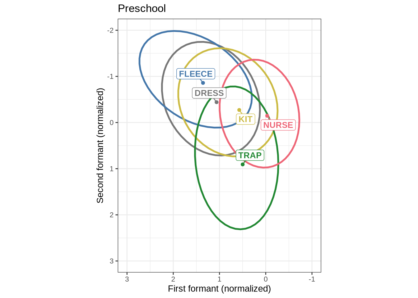
3.2 QuakeBox
In order to interpret Figure 1, it is worth looking at adults from the same community on the same scale.
QB1_summary <- QB1 |>
  filter(
    vowel %in% short_front,
    !unstressed
  ) |>
  group_by(vowel) |>
  summarise(
    mean_f1 = mean(F1_lob2),
    mean_f2 = mean(F2_lob2)
  )

QB1_mean_plot <- QB1 |>
  filter(
    vowel %in% short_front,
    !unstressed
  ) |>
  ggplot(
    aes(
      x = F2_lob2,
      y = F1_lob2,
      colour = vowel,
      label = vowel
    )
  ) +
  stat_ellipse(level=0.68, linewidth=1) +
  geom_point(data = QB1_summary, aes(x=mean_f2, y=mean_f1)) +
  geom_label_repel(
    mapping = aes(x=mean_f2, y=mean_f1),
    min.segment.length = 0, seed = 42,
    show.legend = FALSE,
    fontface = "bold",
    size = 10 / .pt,
    max.overlaps = Inf,
    force = 2,
    label.padding = unit(0.2, "lines"),
    data = QB1_summary
  ) +
  scale_x_reverse(limits = c(3, -1)) +
  scale_y_reverse(limits = c(3, -2)) +
  scale_colour_manual(values = vowel_colours_5) +
  coord_fixed() +
  theme(
    legend.position = "none"
  ) +
  labs(
    title = "Community (QuakeBox)",
    x = "First formant (normalized)",
    y = "Second formant (normalized)"
  )

QB1_mean_plot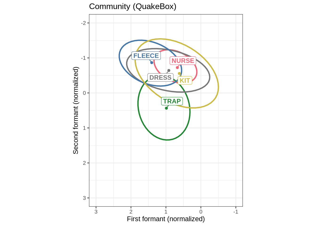
We now combine Figure 1 and Figure 2 into a single plot and save it to become Figure 6 in the paper.
combined_raw_plot <- (mean_plot + theme(legend.position = "none")) +
  QB1_mean_plot

ggsave(
  here('plots', 'figure8_normalised_vowel_spaces.tiff'),
  plot = combined_raw_plot,
  width = 7,
  height = 5,
  dpi = 500
)

combined_raw_plot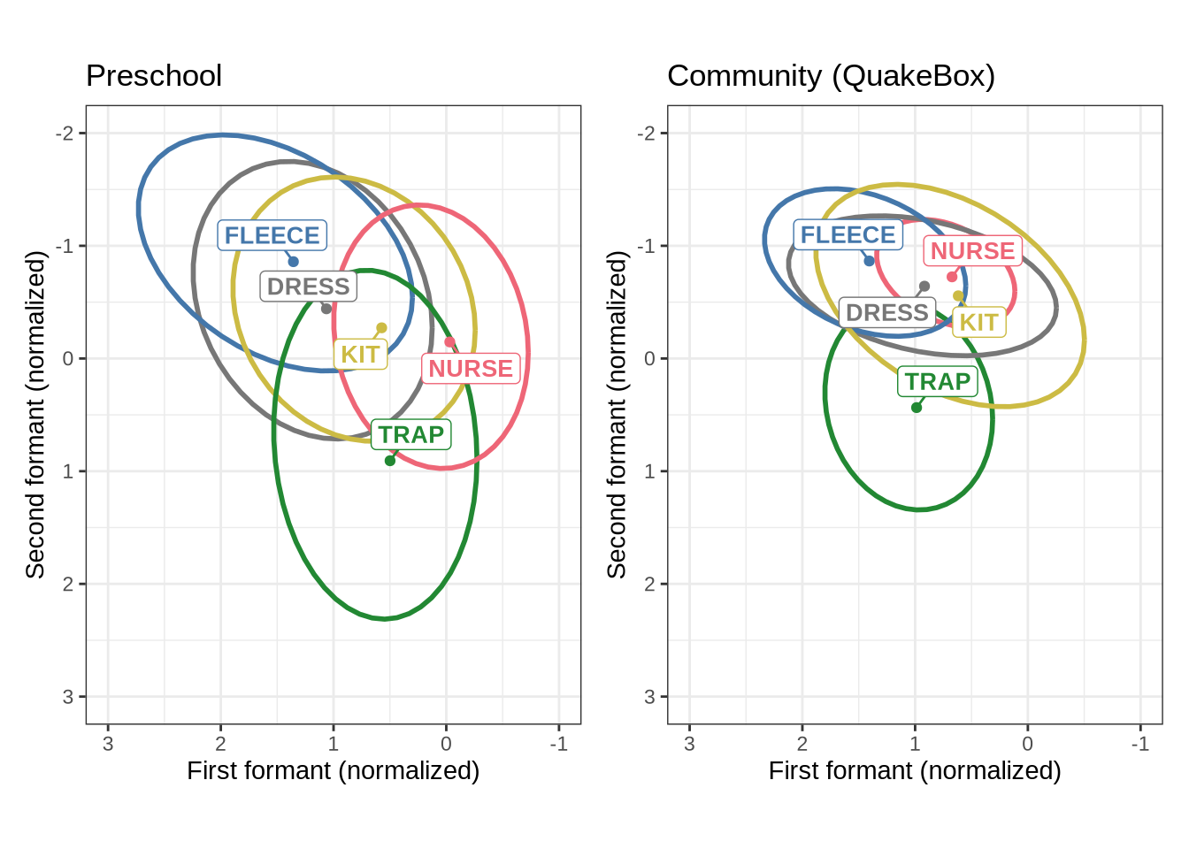
The most obvious feature of Figure 3 is that the kids have much more variability in their production in normalised space. The second thing to note is the higher and fronter position of dress in the preschool data along with the lower and backer trap. The position of nurse is also quite different across the two populations.
4 Modelling
4.1 Preschoolers
4.1.1 Modelling strategy
As noted above, we will be fitting Bayesian GAMMs. The rationale for this is discussed in the paper. Our primary motivation is the increased control over model convergence which Bayesian methods allow. This comes, in part, from the capacity to set informative priors and to specify the underlying probabilistic model we assume.
Our model structure is as follows, applied to each vowel-formant separately (e.g. to the normalised first formant of dress):
normalised_formant_values ~ gender + stopword +
    s(age_s, by=gender, k = 5) +
    s(duration_s, k = 5) +
    (1 | w_s) +
    (1 | p_c)
We adopt an apparent time rather than real time approach even though our data has some longitudinal component. We believe that the coverage across each time point for the speakers is insufficient for a good longitudinal model (although one is fit at the end of this document to see if anything emeges which is incompatible with the apparent time approach).
The consequence of this apparent time approach is that age is our primary independent variable. We fit a smooth function for age for each gender in the data set (binary, male and female). We also include stopwords in the data, allowing the model to fit a distinct intercept for each level of ‘stopword’. We fit a smooth function for duration as a proxy for capturing the effect of local speech rate.
The random effects structure we adopt consists of random intercepts for each preschooler, at each collect (1|p_c). That is, the data for the first collection point of a speaker has a distinct random intercept from their second. We also fit a random effect for each word, distinguishing stressed and unstressed syllables from the word (1|w_s). That is, for instance, we allow a random intercept for the stressed syllable in “remember” and another random intercept for tokens coming from the non-stressed syllables (with, as noted above, stress coming from CELEX).
The tag _s indicates that we have scaled the variables.
We use a t-distribution as our response, learning the degrees of freedom parameter from the data. This is means the model is less sensitive to any remaining extreme values in the data.
We use a reasonably conservative prior, designed to aid model convergence while allowing a wide range of formant values to be capture by the model. That is, the only information which we try to incorporate in to the prior is that we are predicting normalised formant values. More detail is provided in the prior predictive check below.
We now fit models to each vowel. There is a distinct tab for each vowel, each of which contains a model for normalised F1 and F2. We begin with the prior predictive check (to ensure the prior does not exclude plausible values).
We fit with 4 chains and 3000 iterations. We start with adapt_delta=0.9. This is the step size when exploring the probability distribution. We reduce it for models which report divergent transitions.
4.1.2 By-vowel
We begin by sampling from our prior distribution to ensure that we are producing values in the ballpark of plausible values for our data. We’ll fit this using the data for dress. This is for coding convenience, as the model is not learning from the data. What we are doing here is ensuring that we are not unduly biasing the model towards a particular result.
dress_f1_data <- f1 |>
  filter(
    vowel == "DRESS"
  ) |>
  mutate(
    w_s = interaction(word, stressed),
    p_c = interaction(participant, collect)
  ) %>%
  droplevels()
We establish the prior distribution and take samples from it.
prior_t <- c(
  prior(gamma(2, 3), class = "nu"), # degrees of freedom of t-distribution
  prior(exponential(1), class = "sigma"), # variance parameter for t-distribution
  prior(normal(0, 2), class = "Intercept"), # global intercept value (at reference level).
  prior(normal(0, 1), class = "sd"), # sd for random intercept terms.
  prior(normal(0, 0.5), class = "sds"), # smoothing parameters (how wiggly)
  prior(normal(0, 2), class = "b") # fixed effects coefficients
)
dress_f1_prior_t <- brm(
F1_lob2 ~ gender + stopword +
s(age_s, by=gender, k = 5) +
s(duration_s, k = 5) +
(1 | w_s) +
(1 | p_c),
data = dress_f1_data,
family = student(),
prior = prior_t,
chains = 4,
cores = 4,
iter = 2000,
control = list(adapt_delta = 0.9),
sample_prior = "only"
)
write_rds(
dress_f1_prior_t,
here('models', 'dress_f1_prior_t.rds'),
compress = "gz"
)We take 100 draws from the prior and plot the distribution.
prior_draws <- posterior_predict(dress_f1_prior_t, ndraws = 100)
prior_draws <- prior_draws |>
  t() |>
  as_tibble(.name_repair='unique') |>
  bind_cols(dress_f1_data) |>
  pivot_longer(
    cols = contains('...'),
    names_to = "draw_index",
    values_to = "draw_value"
  ) |>
  mutate(
    draw_index = as.numeric(str_replace(draw_index, "...", ""))
  )

prior_draws |>
  ggplot(
    aes(
      x = age_s,
      y = draw_value
    )
  ) +
  geom_jitter(alpha = 0.1) +
  geom_smooth() +
  labs(
    title = "100 draws from the prior predictive distribution"
  ) +
  scale_y_continuous(limits=c(-20, 20))
What we want to see here is that our prior is not excluding plausible values. If anything, our prior could be made even more informative (i.e. restrict the results more). But this should be sufficient for present purposes.
4.1.2.0.1 F1
We repeat the code to extract the dress data so that this tab matches the tabs for the other vowels (i.e. the following block is repeated from the start of the prior predictive check tab).
dress_f1_data <- f1 |>
  filter(
    vowel == "DRESS"
  ) |>
  mutate(
    w_s = interaction(word, stressed),
    p_c = interaction(participant, collect)
  ) %>%
  droplevels()


summary(dress_f1_data)
participant collect age_s gender word
Length:945 Min. :1.000 Min. :-1.83828 F:531 then :475
Class :character 1st Qu.:2.000 1st Qu.:-0.84298 M:414 went : 80
Mode :character Median :3.000 Median :-0.09651 said : 77
Mean :2.666 Mean :-0.08124 nest : 44
3rd Qu.:4.000 3rd Qu.: 0.64996 better : 31
Max. :4.000 Max. : 2.14290 remember: 27
(Other) :211
vowel stressed stopword F1_lob2
DRESS:945 Mode :logical Mode :logical Min. :-3.6074
FALSE:36 FALSE:356 1st Qu.:-1.1944
TRUE :909 TRUE :589 Median :-0.7474
Mean :-0.5646
3rd Qu.:-0.0281
Max. : 4.3793
duration_s age w_s p_c
Min. :-0.8999 Min. :47.00 then.TRUE :457 EC0919-Child.1: 23
1st Qu.:-0.5655 1st Qu.:51.00 went.TRUE : 80 EC0105-Child.2: 22
Median :-0.2499 Median :54.00 said.TRUE : 74 EC2432-Child.3: 20
Mean :-0.1059 Mean :54.06 nest.TRUE : 44 EC0503-Child.2: 19
3rd Qu.: 0.1844 3rd Qu.:57.00 better.TRUE : 29 EC0501-Child.2: 18
Max. : 2.4698 Max. :63.00 remember.TRUE: 26 EC0501-Child.1: 17
(Other) :235 (Other) :826 Unsurprisingly, the majority of the words here are stop words. In fact, 480 tokens of 940 are the word ‘then’.
We fit our model for dress
dress_f1_fit <- brm(
    F1_lob2 ~ gender + stopword +
      s(age_s, by=gender, k = 5) +
      s(duration_s, k = 5) +
      (1 | w_s) +
      (1 | p_c),
    data = dress_f1_data,
    family = student(),
    prior = prior_t,
    chains = 4,
    cores = 4,
    iter = 3000,
    control = list(adapt_delta = 0.99),
  )

write_rds(
  dress_f1_fit,
  here('models', 'dress_f1_fit_t.rds'),
  compress = "gz"
)
Let’s look at the model summary.
summary(dress_f1_fit) Family: student
Links: mu = identity; sigma = identity; nu = identity
Formula: F1_lob2 ~ gender + stopword + s(age_s, by = gender, k = 5) + s(duration_s, k = 5) + (1 | w_s) + (1 | p_c)
Data: dress_f1_data (Number of observations: 945)
Draws: 4 chains, each with iter = 3000; warmup = 1500; thin = 1;
total post-warmup draws = 6000
Smoothing Spline Hyperparameters:
Estimate Est.Error l-95% CI u-95% CI Rhat Bulk_ESS
sds(sage_sgenderF_1) 0.32 0.25 0.01 0.93 1.00 2761
sds(sage_sgenderM_1) 0.36 0.27 0.02 1.00 1.00 2669
sds(sduration_s_1) 0.49 0.28 0.04 1.11 1.00 2252
Tail_ESS
sds(sage_sgenderF_1) 2033
sds(sage_sgenderM_1) 2819
sds(sduration_s_1) 1427
Multilevel Hyperparameters:
~p_c (Number of levels: 180)
Estimate Est.Error l-95% CI u-95% CI Rhat Bulk_ESS Tail_ESS
sd(Intercept) 0.48 0.04 0.40 0.57 1.00 1722 2989
~w_s (Number of levels: 66)
Estimate Est.Error l-95% CI u-95% CI Rhat Bulk_ESS Tail_ESS
sd(Intercept) 0.19 0.07 0.05 0.34 1.00 1383 1363
Regression Coefficients:
Estimate Est.Error l-95% CI u-95% CI Rhat Bulk_ESS Tail_ESS
Intercept -0.55 0.09 -0.72 -0.38 1.00 2774 3951
genderM -0.05 0.10 -0.24 0.13 1.00 1938 3014
stopwordTRUE -0.04 0.12 -0.29 0.19 1.00 2335 3084
sage_s:genderF_1 -0.61 0.64 -1.79 0.85 1.00 2610 3246
sage_s:genderM_1 -0.60 0.70 -1.97 0.83 1.00 2836 3494
sduration_s_1 0.60 0.64 -0.71 1.86 1.00 3736 4126
Further Distributional Parameters:
Estimate Est.Error l-95% CI u-95% CI Rhat Bulk_ESS Tail_ESS
sigma 0.57 0.03 0.52 0.63 1.00 2843 4247
nu 3.48 0.48 2.67 4.51 1.00 3616 4602
Draws were sampled using sampling(NUTS). For each parameter, Bulk_ESS
and Tail_ESS are effective sample size measures, and Rhat is the potential
scale reduction factor on split chains (at convergence, Rhat = 1).The above values don’t tell us much by themselves.
We’ll look at some posterior predictive checks to help test that our model is compatible with the data.
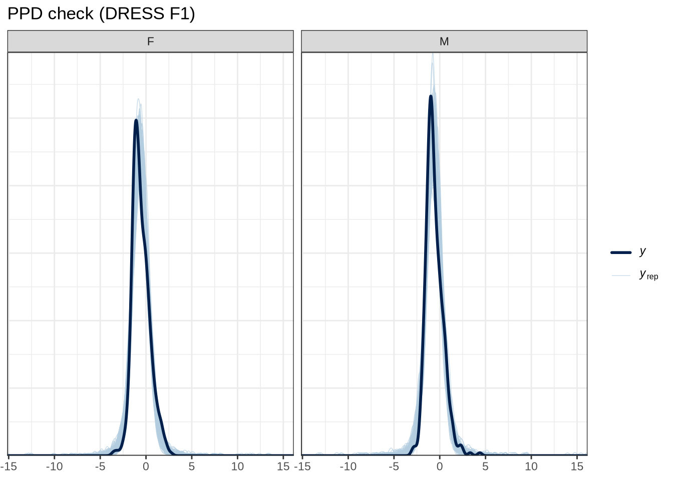
pp_check(dress_f1_fit, type="dens_overlay_grouped", group="gender", ndraws = 100) +
  labs(
    title = "PPD check (DRESS F1)"
  )
pp_check(dress_f1_fit, type = "stat_2d", stat = c("min", "max"), ndraws = 100) +
  labs(
    title = "PPD check (DRESS F1)"
  )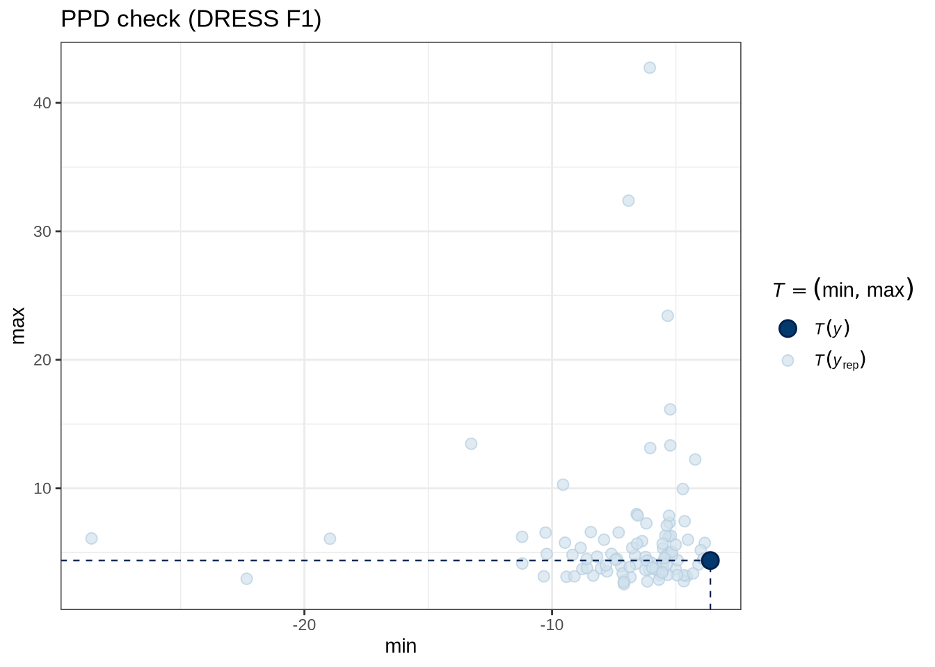
Figure 5 tells us that the actual data (the thick blue point) fits roughly within the range of predictions from our model.
Let’s look at a traditional quantile-quantile plot to assess model predictions.
dress_f1_data %>%
  add_residual_draws(dress_f1_fit) %>%
  median_qi() %>%
  ggplot(aes(sample = .residual)) +
  geom_qq() +
  geom_qq_line()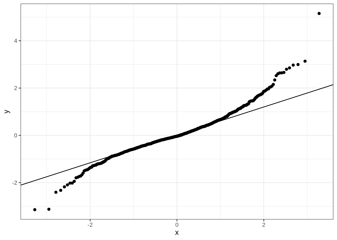
There’s a bit of difficulty in the tails, but nothing too upsetting.
The following block allows us to check model predictions against the longitudinal aspect of the data set. We calculate the mean values for each collection point for each preschooler. We can then determine the difference between collection points in terms of change in mean formant values and change in age. We then calculate the model predictions for the corresponding age values (including the random intercepts for the relevant preschooler and collection points). We then compare the two distributions visually.
diff_check <- function(mod, data) {
  differences <- data %>%
    rename(
      F_lob2 = matches("F[12]_lob2")
    ) %>%
  group_by(participant, collect) %>%
  summarise(
    F_lob2 = mean(F_lob2, na.rm = T),
    age_s = first(age_s),
    gender = first(gender)
  ) %>%
  group_by(participant) %>%
  nest() %>%
  mutate(
    diffs = map(
      data,
      ~ {
        in_dat <- .x %>%
          arrange(age_s)

        out_dat <-
          crossing(
            "age_1" = in_dat$age_s,
            "age_2" = in_dat$age_s,
          ) %>%
          filter(
            age_1 < age_2
          ) %>%
          # get F1 for each.
          left_join(
            in_dat %>%
              rename(age_1 = age_s, F_1 = F_lob2, collect_1 = collect),
            by = "age_1"
          ) %>%
          left_join(
            in_dat %>%
              # get gender from the first one.
              select(-gender) %>%
              rename(age_2 = age_s, F_2 = F_lob2, collect_2 = collect),
            by = "age_2"
          ) %>%
          mutate(
            diff = F_2 - F_1
          )
        out_dat
      }
    )
  ) %>%
  select(-data) %>%
  unnest(diffs)

  age_1_preds <- differences %>%
    rename(
      age_s = age_1,
      collect = collect_1
    ) %>%
    mutate(
      w_s = "nonword",
      duration_s = 0,
      stopword = TRUE
    ) %>%
    ungroup() %>%
    # Basic idea: take 100 draws then take the mean.
    add_epred_draws(
      object = mod,
      ndraws = 100,
      allow_new_levels = TRUE
    ) %>%
    group_by(participant) %>%
    summarise(
      age_1 = first(age_s),
      collect_1 = first(collect),
      gender = first(gender),
      F_1 = mean(.epred)
    )

  age_2_preds <- differences %>%
    rename(
      age_s = age_2,
      collect = collect_2
    ) %>%
    mutate(
      w_s = "nonword",
      duration_s = 0,
      stopword = TRUE
    ) %>%
    ungroup() %>%
    add_epred_draws(
      object = mod,
      ndraws = 100,
      allow_new_levels = TRUE
    ) %>%
    group_by(participant) %>%
    summarise(
      age_2 = first(age_s),
      collect_2 = first(collect),
      gender = first(gender),
      F_2 = mean(.epred)
    )

  all_diffs <- bind_rows(
    "data" = differences,
    "preds" = left_join(
        age_1_preds,
        age_2_preds,
        by = c("participant", "gender")
      ) %>%
      mutate(diff = F_2 - F_1),
    .id = "source"
  )

  all_diffs
}

diff_plot <- function(all_diffs) {
  all_diffs %>%
    ggplot(
      aes(
        fill = source,
        colour = source,
        x = diff
      )
    ) +
    geom_density(alpha = 0.2) +
    geom_vline(
      aes(
        xintercept = mean_diff,
        colour = source
      ),
      data = ~ .x %>% group_by(source, gender) %>% summarise(mean_diff = mean(diff))
    ) +
    facet_wrap(vars(gender))
}


diff_check(dress_f1_fit, dress_f1_data) %>%
  diff_plot()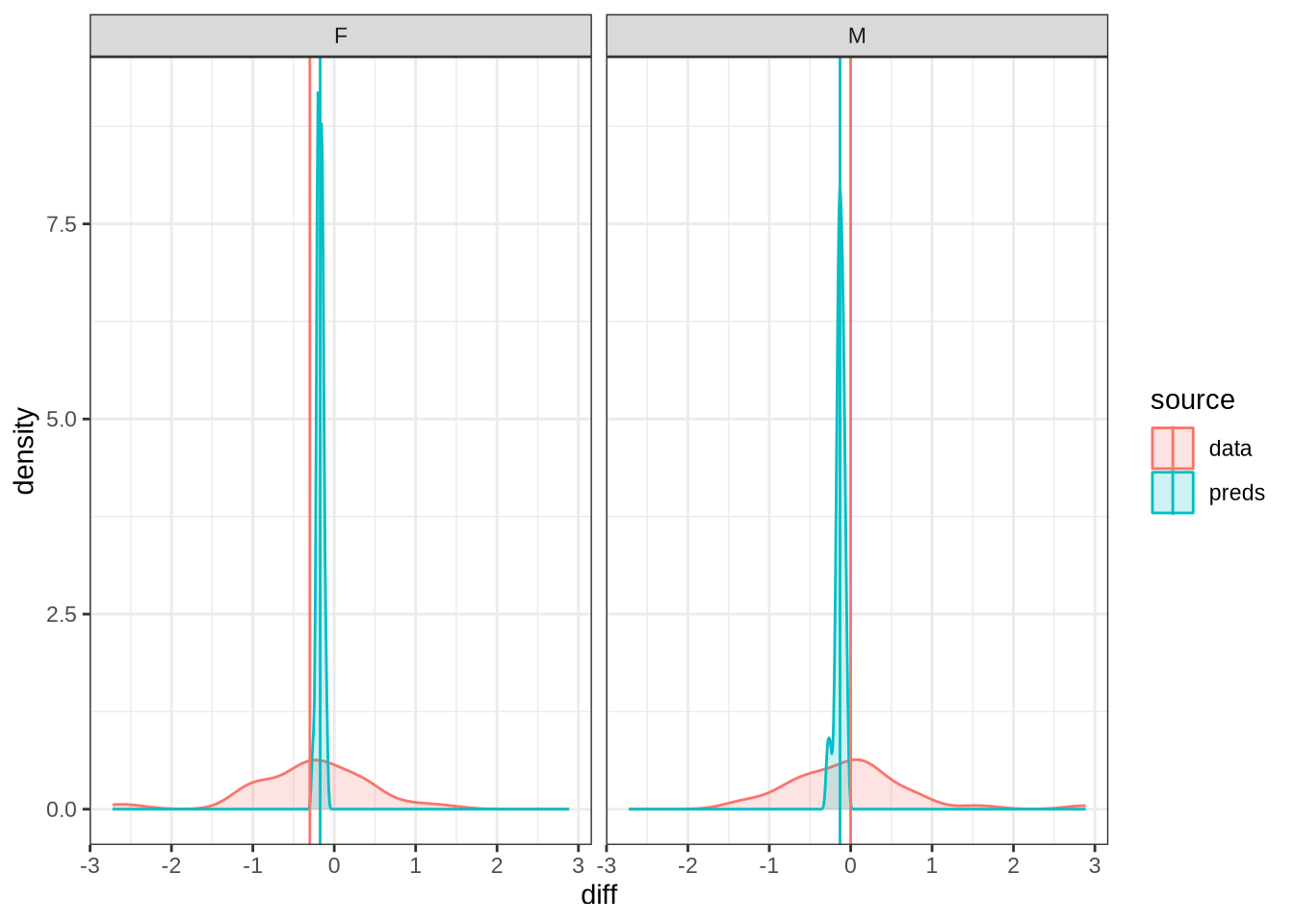
Figure 7 displays the distribution of predicted values across 100 draws from the posterior distribution (blue) for each difference between collection points in the real data (red). The horizontal lines indicate the mean difference between collection subsequent collection points as predicted (blue) and actually measured (red). We facet by gender.
A model which fully captured all the sources of variation in the changes in formant values between collection points would have the an overlapping distribution here. That is not the case here. Our model obviously does not capture some of this variation (perhaps this is unsurprising as we don’t directly model it!). Looking at the vertical lines, we seem to be underestimating the vowel space rising for female preschoolers and slightly overestimating the (very small) mean change in the male preschoolers.
We now plot smooths for both male and female preschoolers using the modelbased package to generate predictions across both age and duration.
First, duration:
estimate_relation(dress_f1_fit, by = "duration_s", predict="link", ci = 0.9) %>%
  plot() +
  scale_y_reverse()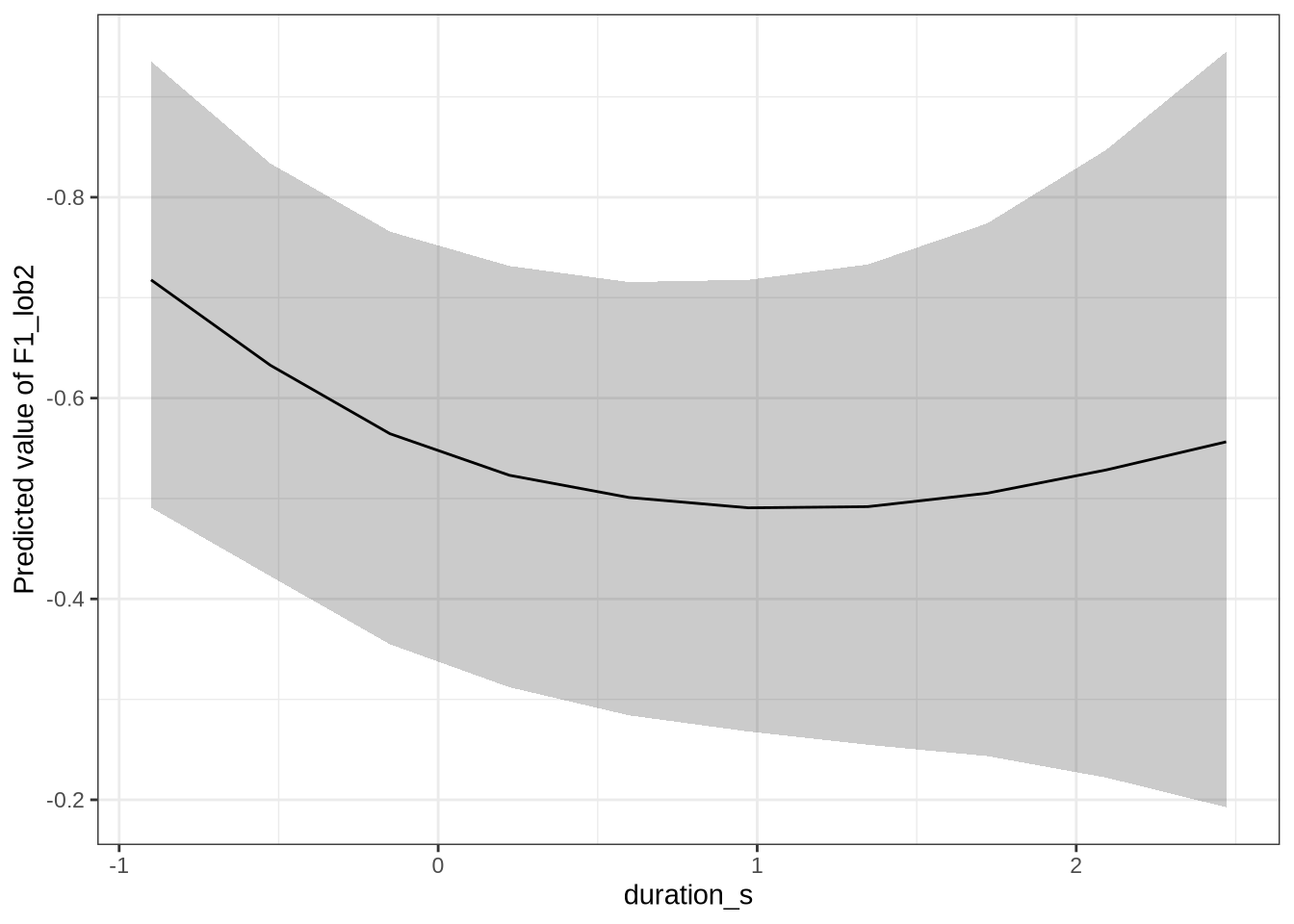
This is not the pattern we expect. As the duration of the vowel increases, it gets lower in the vowel space (note, reversed y-axis!). As a stand-in for speech rate, this is not what we expect. That is, with slower speech, we’d expect less reduction, and so a higher and fronter dress. Note the large confidence bars, though.
dress_f1_preds <- estimate_relation(
    dress_f1_fit,
    by = list(
      age_s = seq(min_age_s, max_age_s, length = 50),
      gender = c("F", "M"),
      duration_s = 0
    ),
    predict="link",
    ci = c(0.9, 0.7)
  )

dress_f1_preds %>%
  plot() +
  scale_y_reverse()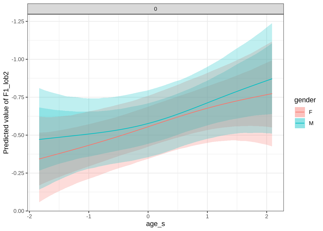
In Figure 9, the \(y\)-axis is flipped, so that a rising line indicates a rising vowel in the vowel space. We see that, for the female children, there is a steady rise in the dress, albeit with wide error bars. We plot both the 70% and 90% credible intervals to give a more graded sense of model uncertainty.
For our convenience for subsequent models, the following function generates all the smooth plots we are interested in. This time, just with a 90% interval.
# This model uses the original `kids` dataframe as a global variable.
# Not good programming practice, but convenient in this case.
model_plots <- function(model) {
  dur_plot <-
    estimate_relation(
      model,
      by = "duration_s",
      predict="link", ci = 0.9
    ) %>%
    plot() +
    scale_y_reverse()

  age_plot <-
    estimate_relation(
      model,
      by = c("age_s", "gender", "duration_s = 0"),
      predict="link",
      ci = 0.9
    ) %>%
    plot() +
    scale_y_reverse()


  age_plot + dur_plot
}
Test it’s what we expect:
model_plots(dress_f1_fit) + plot_annotation(
  title = "DRESS F1"
)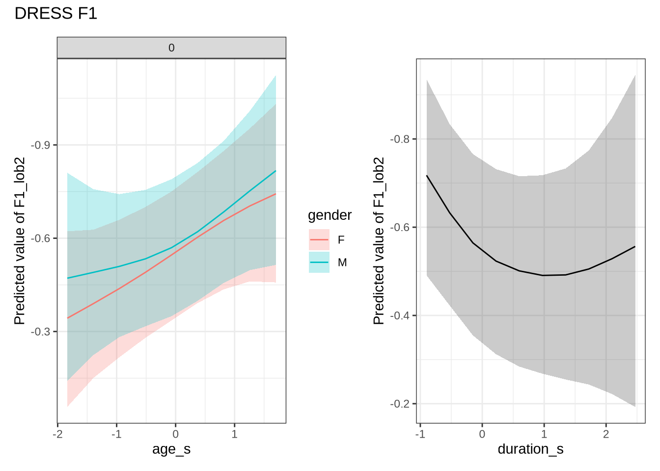
Looking good.
For dress, fleece and kit we report a distribution for difference between 50 months and 60 months. In this supplementary document, we’ll provide this for all models.
# Want to take samples from 50 months and 60 months.
sample_points = c(
  ## What are 50 and 60 in age_s?
  (50 - mean(kids$age)) / sd(kids$age),
  # = -1.09
  (60 - mean(kids$age)) / sd(kids$age)
  # = 1.4
)

ten_month_preds <- function(mod, sample_points) {
  preds <-
    expand_grid(
      "age_s" = sample_points,
      "gender" = c("F", "M"),
    ) %>%
    mutate(
      stopword = FALSE,
      duration_s = 0,
      w_s = "not",
      p_c = "real"
    ) |>
    add_epred_draws(
      mod,
      re_formula = NA,
      allow_new_levels=TRUE,
      ndraws=1000
    ) %>%
    ungroup() %>%
    mutate(
      age = if_else(
        between(age_s, sample_points[[1]]-0.01, sample_points[[1]]+0.01),
        "m50",
        "m60"
      )
    ) %>%
    select(.draw, gender, age, .epred) %>%
    pivot_wider(
      names_from = age,
      values_from = .epred
    ) %>%
    mutate(
      .draw = .draw,
      gender = gender,
      diff = m60 - m50,
      .keep = "none"
    )
}

dress_f1_10 <- ten_month_preds(dress_f1_fit, sample_points)

dress_f1_10 %>%
  ggplot(
    aes(
      x = diff,
      colour = gender,
      fill = gender
    )
  ) +
  geom_density(linewidth = 1, alpha = 0.2) +
  geom_vline(xintercept = 0, linetype = "dashed")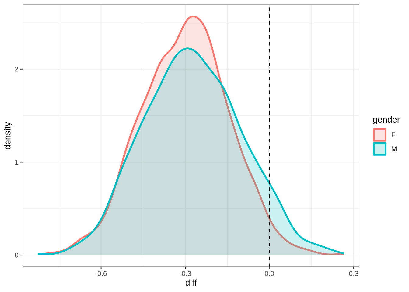
Now we move on to the second formant.
4.1.2.0.2 F2
dress_f2_data <- f2 |>
  filter(
    vowel == "DRESS"
  ) |>
  mutate(
    w_s = interaction(word, stressed),
    p_c = interaction(participant, collect)
  ) %>%
  droplevels()

summary(dress_f2_data)
participant collect age_s gender word
Length:940 Min. :1.000 Min. :-1.83828 F:536 then :478
Class :character 1st Qu.:2.000 1st Qu.:-0.84298 M:404 said : 80
Mode :character Median :3.000 Median :-0.09651 went : 65
Mean :2.648 Mean :-0.09228 nest : 47
3rd Qu.:4.000 3rd Qu.: 0.64996 better : 31
Max. :4.000 Max. : 2.14290 remember: 25
(Other) :214
vowel stressed stopword F2_lob2
DRESS:940 Mode :logical Mode :logical Min. :-1.617
FALSE:36 FALSE:345 1st Qu.: 0.673
TRUE :904 TRUE :595 Median : 1.206
Mean : 1.133
3rd Qu.: 1.697
Max. : 4.790
duration_s age w_s p_c
Min. :-0.89992 Min. :47.00 then.TRUE :460 EC0919-Child.1: 23
1st Qu.:-0.53849 1st Qu.:51.00 said.TRUE : 77 EC0105-Child.2: 22
Median :-0.19372 Median :54.00 went.TRUE : 65 EC2432-Child.3: 20
Mean :-0.07502 Mean :54.02 nest.TRUE : 47 EC0501-Child.2: 18
3rd Qu.: 0.22521 3rd Qu.:57.00 better.TRUE : 29 EC0503-Child.2: 18
Max. : 2.46981 Max. :63.00 remember.TRUE: 24 EC0501-Child.1: 17
(Other) :238 (Other) :822 dress_f2_fit <- brm(
F2_lob2 ~ gender + stopword +
s(age_s, by=gender, k = 5) +
s(duration_s, k = 5) +
(1 | w_s) +
(1 | p_c),
data = dress_f2_data,
family = student(),
prior = prior_t,
chains = 4,
cores = 4,
iter = 3000,
control = list(adapt_delta = 0.99),
)
write_rds(
dress_f2_fit,
here('models', 'dress_f2_fit_t.rds'),
compress = "gz"
)dress_f2_fit <- read_rds(here('models', 'dress_f2_fit_t.rds'))summary(dress_f2_fit) Family: student
Links: mu = identity; sigma = identity; nu = identity
Formula: F2_lob2 ~ gender + stopword + s(age_s, by = gender, k = 5) + s(duration_s, k = 5) + (1 | w_s) + (1 | p_c)
Data: dress_f2_data (Number of observations: 940)
Draws: 4 chains, each with iter = 3000; warmup = 1500; thin = 1;
total post-warmup draws = 6000
Smoothing Spline Hyperparameters:
Estimate Est.Error l-95% CI u-95% CI Rhat Bulk_ESS
sds(sage_sgenderF_1) 0.32 0.25 0.01 0.93 1.00 2933
sds(sage_sgenderM_1) 0.33 0.26 0.01 0.96 1.00 4066
sds(sduration_s_1) 0.41 0.26 0.02 1.02 1.00 3228
Tail_ESS
sds(sage_sgenderF_1) 3099
sds(sage_sgenderM_1) 3254
sds(sduration_s_1) 2947
Multilevel Hyperparameters:
~p_c (Number of levels: 181)
Estimate Est.Error l-95% CI u-95% CI Rhat Bulk_ESS Tail_ESS
sd(Intercept) 0.42 0.04 0.35 0.50 1.00 1731 3165
~w_s (Number of levels: 68)
Estimate Est.Error l-95% CI u-95% CI Rhat Bulk_ESS Tail_ESS
sd(Intercept) 0.41 0.07 0.29 0.56 1.00 2091 3387
Regression Coefficients:
Estimate Est.Error l-95% CI u-95% CI Rhat Bulk_ESS Tail_ESS
Intercept 1.09 0.10 0.90 1.28 1.00 3420 4680
genderM 0.00 0.08 -0.16 0.16 1.00 2747 3601
stopwordTRUE 0.12 0.19 -0.24 0.49 1.00 2382 3223
sage_s:genderF_1 0.35 0.65 -0.83 1.84 1.00 3298 3769
sage_s:genderM_1 0.40 0.67 -0.89 1.77 1.00 3691 4042
sduration_s_1 0.70 0.57 -0.35 1.99 1.00 5382 4149
Further Distributional Parameters:
Estimate Est.Error l-95% CI u-95% CI Rhat Bulk_ESS Tail_ESS
sigma 0.42 0.03 0.37 0.47 1.00 2756 3878
nu 2.37 0.27 1.90 2.95 1.00 4373 4821
Draws were sampled using sampling(NUTS). For each parameter, Bulk_ESS
and Tail_ESS are effective sample size measures, and Rhat is the potential
scale reduction factor on split chains (at convergence, Rhat = 1).We won’t explicitly comment on plots unless something striking emerges.
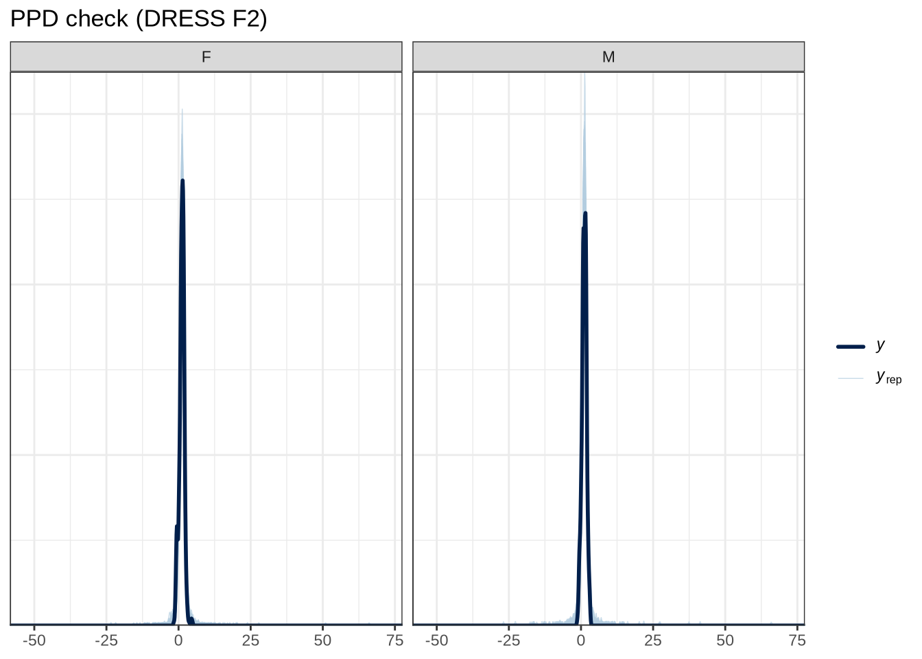
pp_check(dress_f2_fit, type="dens_overlay_grouped", group="gender", ndraws = 100) +
  labs(
    title = "PPD check (DRESS F2)"
  )
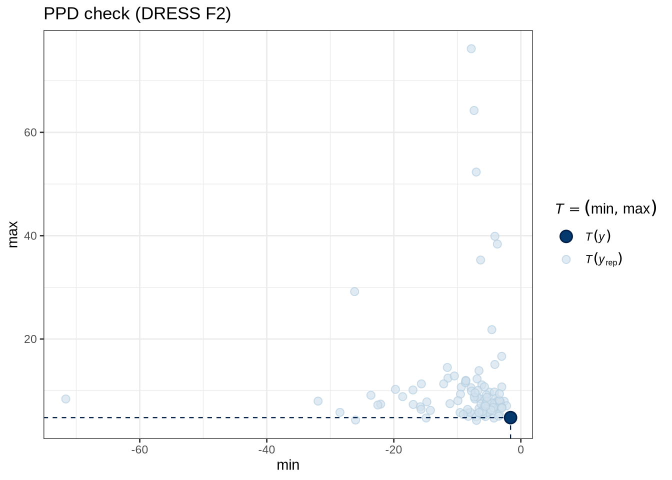
pp_check(dress_f2_fit, type = "stat_2d", stat = c("min", "max"), ndraws = 100) +
  labs(
    title = "PPD check (DRESS F2)"
  )
dress_f2_data %>%
  add_residual_draws(dress_f2_fit) %>%
  median_qi() %>%
  ggplot(aes(sample = .residual)) +
  geom_qq() +
  geom_qq_line()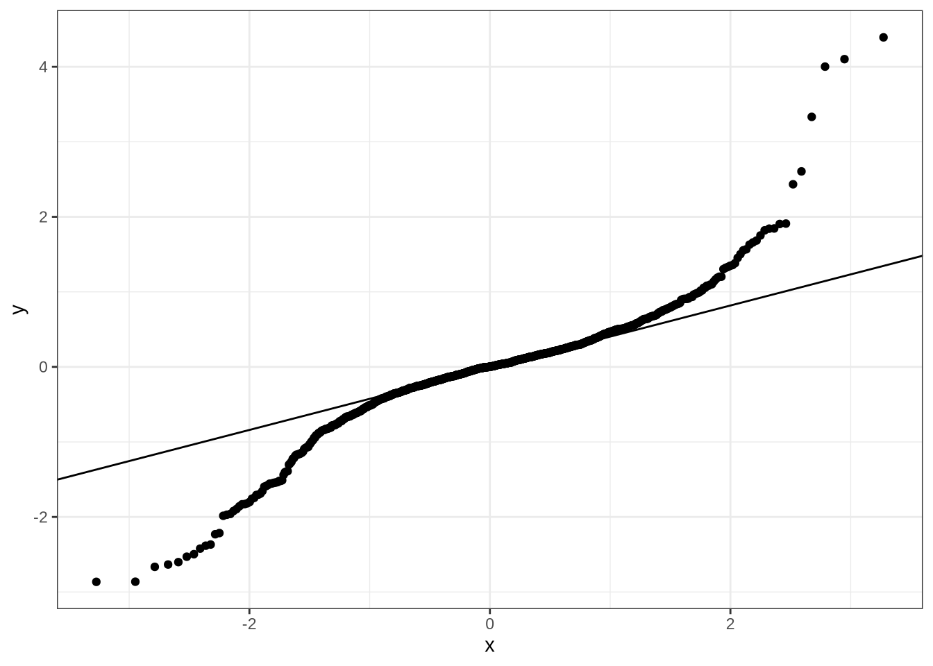
model_plots(dress_f2_fit) +
  plot_annotation(title = "DRESS F2")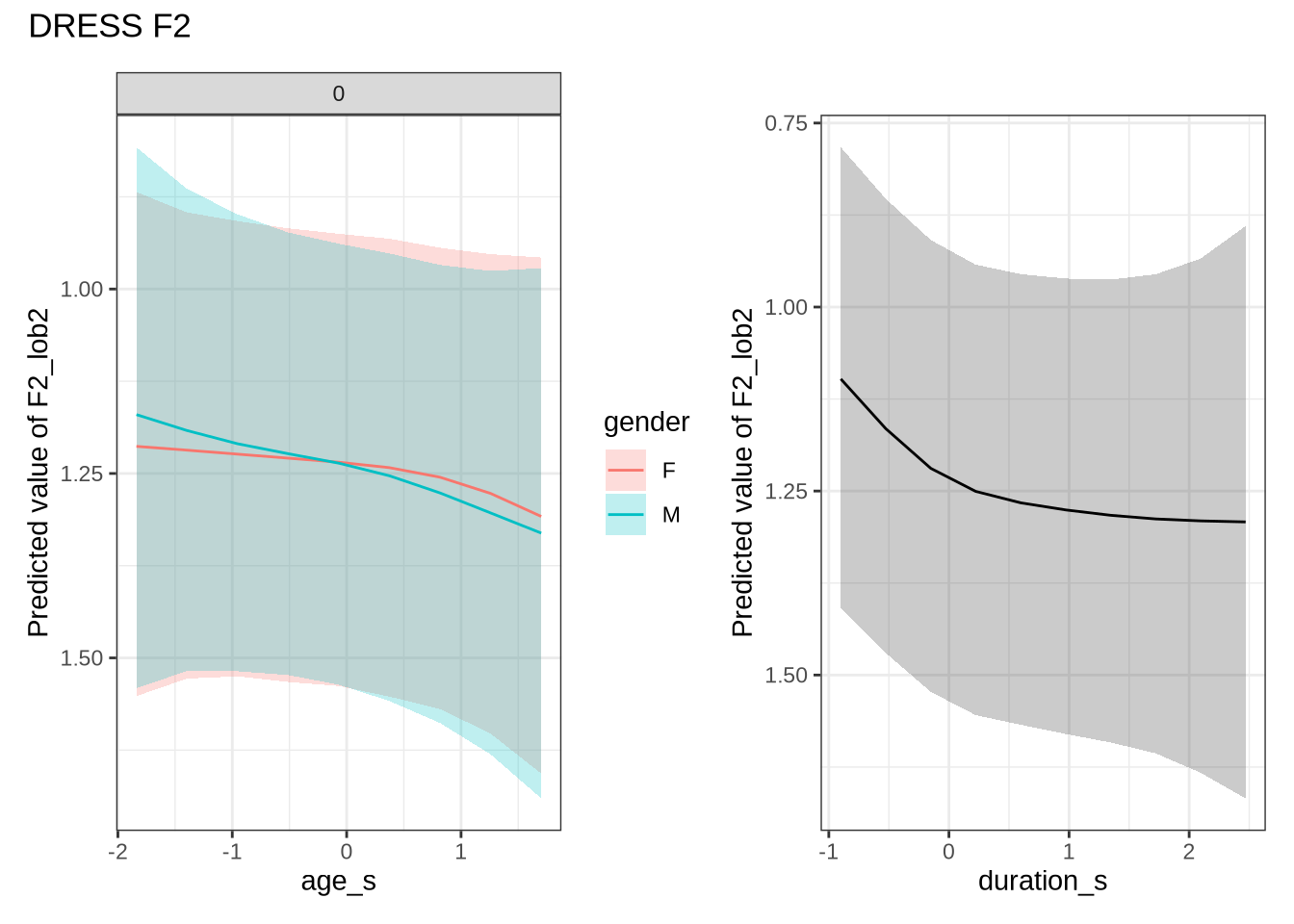
No change which we can be confident of predicted here.
We generate predictions.
dress_f2_preds <- estimate_relation(
    dress_f2_fit,
    by = list(
      age_s = seq(min_age_s, max_age_s, length = 50),
      gender = c("F", "M"),
      duration_s = 0
    ),
    predict="link",
    ci = c(0.9, 0.7)
  )
dress_f2_10 <- ten_month_preds(dress_f2_fit, sample_points)
dress_f2_10 %>%
ggplot(
aes(
x = diff,
colour = gender,
fill = gender
)
) +
geom_density(linewidth = 1, alpha = 0.2) +
geom_vline(xintercept = 0, linetype = "dashed")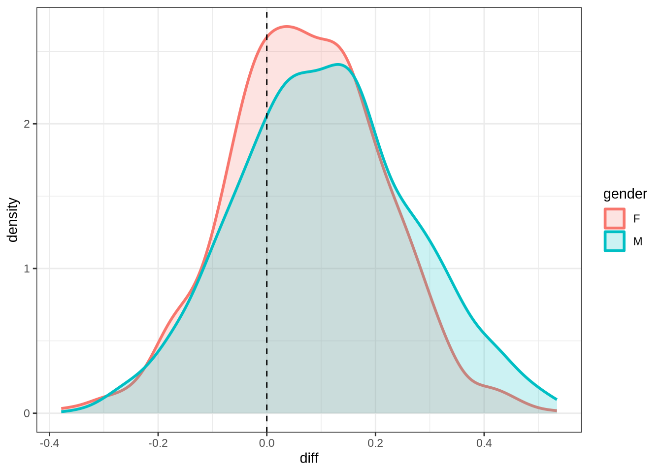
Once we are done with plotting the models for a particular vowel, we remove them from the R environment to free up space for the next models.
rm(dress_f1_fit, dress_f2_fit)4.1.2.0.3 F1
kit_f1_data <- f1 |>
  filter(
    vowel == "KIT"
  ) |>
  mutate(
    w_s = interaction(word, stressed),
    p_c = interaction(participant, collect)
  ) %>%
  droplevels()


summary(kit_f1_data)
participant collect age_s gender word
Length:1837 Min. :1.000 Min. :-1.83828 F:975 his : 211
Class :character 1st Qu.:2.000 1st Qu.:-0.84298 M:862 him : 190
Mode :character Median :3.000 Median : 0.15231 it : 112
Mean :2.801 Mean : 0.05966 bridge : 90
3rd Qu.:4.000 3rd Qu.: 0.89878 the : 87
Max. :4.000 Max. : 2.64055 baby : 65
(Other):1082
vowel stressed stopword F1_lob2
KIT:1837 Mode :logical Mode :logical Min. :-3.57123
FALSE:652 FALSE:1047 1st Qu.:-1.20097
TRUE :1185 TRUE :790 Median :-0.62589
Mean :-0.55152
3rd Qu.: 0.06089
Max. : 5.35072
duration_s age w_s p_c
Min. :-0.8373 Min. :47.00 his.TRUE : 202 EC1402-Child.3: 38
1st Qu.:-0.5859 1st Qu.:51.00 him.TRUE : 175 EC0405-Child.2: 30
Median :-0.2749 Median :55.00 it.TRUE : 109 EC0918-Child.4: 27
Mean :-0.0985 Mean :54.63 bridge.TRUE: 88 EC0901-Child.4: 24
3rd Qu.: 0.1750 3rd Qu.:58.00 the.TRUE : 87 EC0102-Child.4: 23
Max. : 2.4875 Max. :65.00 baby.FALSE : 65 EC2024-Child.1: 22
(Other) :1111 (Other) :1673 kit_f1_fit <- brm(
F1_lob2 ~ gender + stopword +
s(age_s, by=gender, k = 5) +
s(duration_s, k = 5) +
(1 | w_s) +
(1 | p_c),,
data = kit_f1_data,
family = student(),
prior = prior_t,
chains = 4,
cores = 4,
iter = 4000,
control = list(adapt_delta = 0.99),
)
write_rds(
kit_f1_fit,
here('models', 'kit_f1_fit_t.rds'),
compress = "gz"
)kit_f1_fit <- read_rds(here('models', 'kit_f1_fit_t.rds'))summary(kit_f1_fit) Family: student
Links: mu = identity; sigma = identity; nu = identity
Formula: F1_lob2 ~ gender + stopword + s(age_s, by = gender, k = 5) + s(duration_s, k = 5) + (1 | w_s) + (1 | p_c)
Data: kit_f1_data (Number of observations: 1837)
Draws: 4 chains, each with iter = 4000; warmup = 2000; thin = 1;
total post-warmup draws = 8000
Smoothing Spline Hyperparameters:
Estimate Est.Error l-95% CI u-95% CI Rhat Bulk_ESS
sds(sage_sgenderF_1) 0.30 0.23 0.01 0.86 1.00 4151
sds(sage_sgenderM_1) 0.32 0.25 0.01 0.93 1.00 3574
sds(sduration_s_1) 0.48 0.26 0.04 1.06 1.00 2925
Tail_ESS
sds(sage_sgenderF_1) 3851
sds(sage_sgenderM_1) 3707
sds(sduration_s_1) 1901
Multilevel Hyperparameters:
~p_c (Number of levels: 200)
Estimate Est.Error l-95% CI u-95% CI Rhat Bulk_ESS Tail_ESS
sd(Intercept) 0.29 0.03 0.23 0.35 1.00 3288 4933
~w_s (Number of levels: 217)
Estimate Est.Error l-95% CI u-95% CI Rhat Bulk_ESS Tail_ESS
sd(Intercept) 0.44 0.05 0.35 0.53 1.00 2164 4361
Regression Coefficients:
Estimate Est.Error l-95% CI u-95% CI Rhat Bulk_ESS Tail_ESS
Intercept -0.70 0.06 -0.82 -0.58 1.00 3707 5170
genderM -0.05 0.06 -0.16 0.07 1.00 3978 5712
stopwordTRUE 0.25 0.13 -0.01 0.50 1.00 1713 2774
sage_s:genderF_1 0.44 0.57 -0.78 1.61 1.00 4548 4698
sage_s:genderM_1 -0.11 0.59 -1.42 1.00 1.00 4520 4137
sduration_s_1 0.95 0.59 -0.16 2.21 1.00 5234 5604
Further Distributional Parameters:
Estimate Est.Error l-95% CI u-95% CI Rhat Bulk_ESS Tail_ESS
sigma 0.65 0.02 0.61 0.70 1.00 4538 5993
nu 3.93 0.41 3.20 4.82 1.00 6506 6585
Draws were sampled using sampling(NUTS). For each parameter, Bulk_ESS
and Tail_ESS are effective sample size measures, and Rhat is the potential
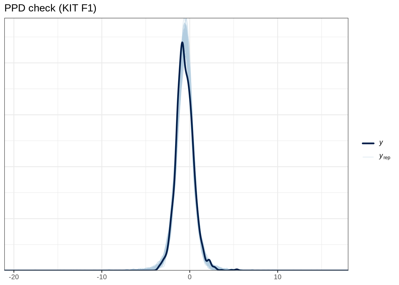
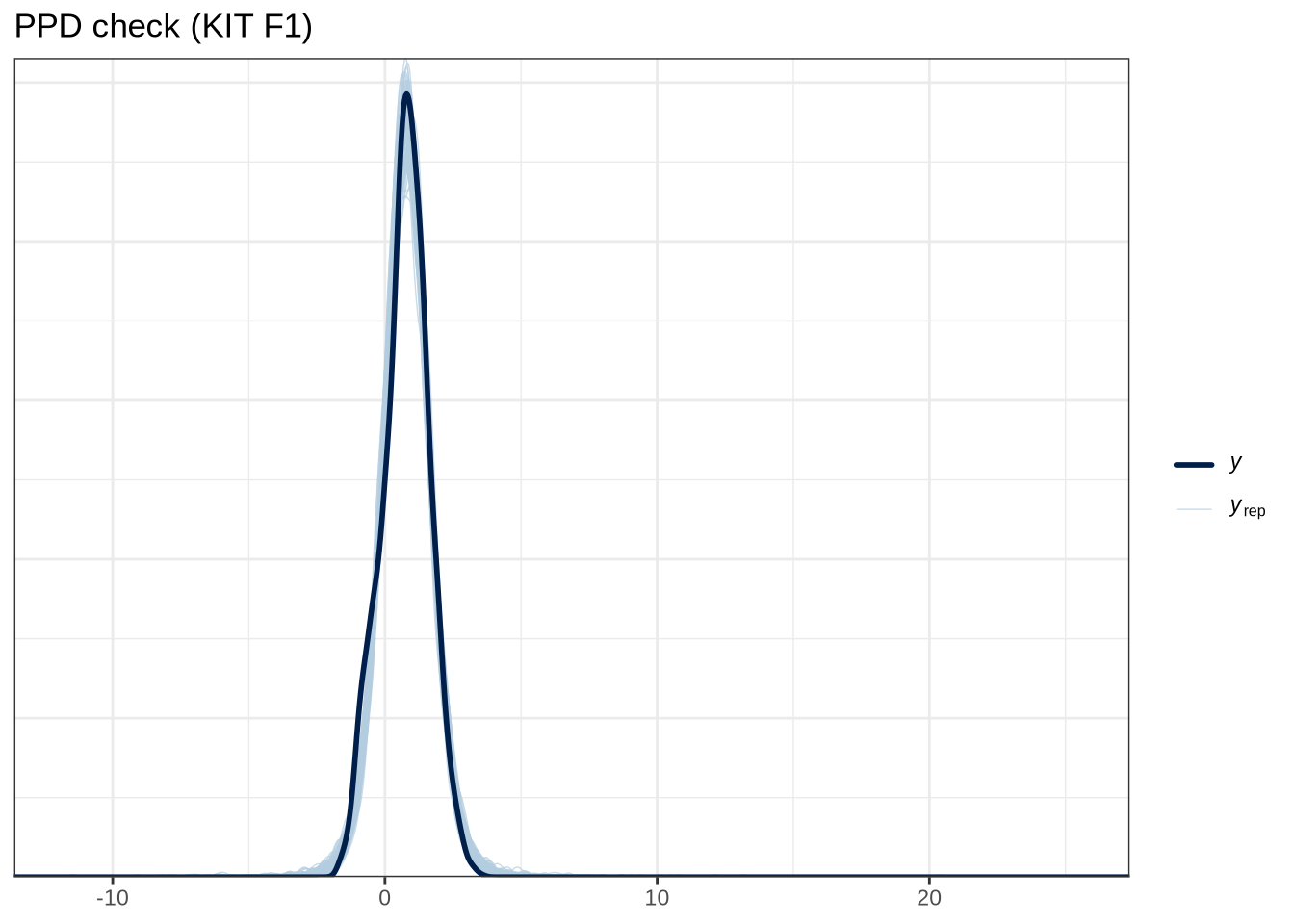
scale reduction factor on split chains (at convergence, Rhat = 1).pp_check(kit_f1_fit, ndraws = 100) +
labs(
title = "PPD check (KIT F1)"
) 
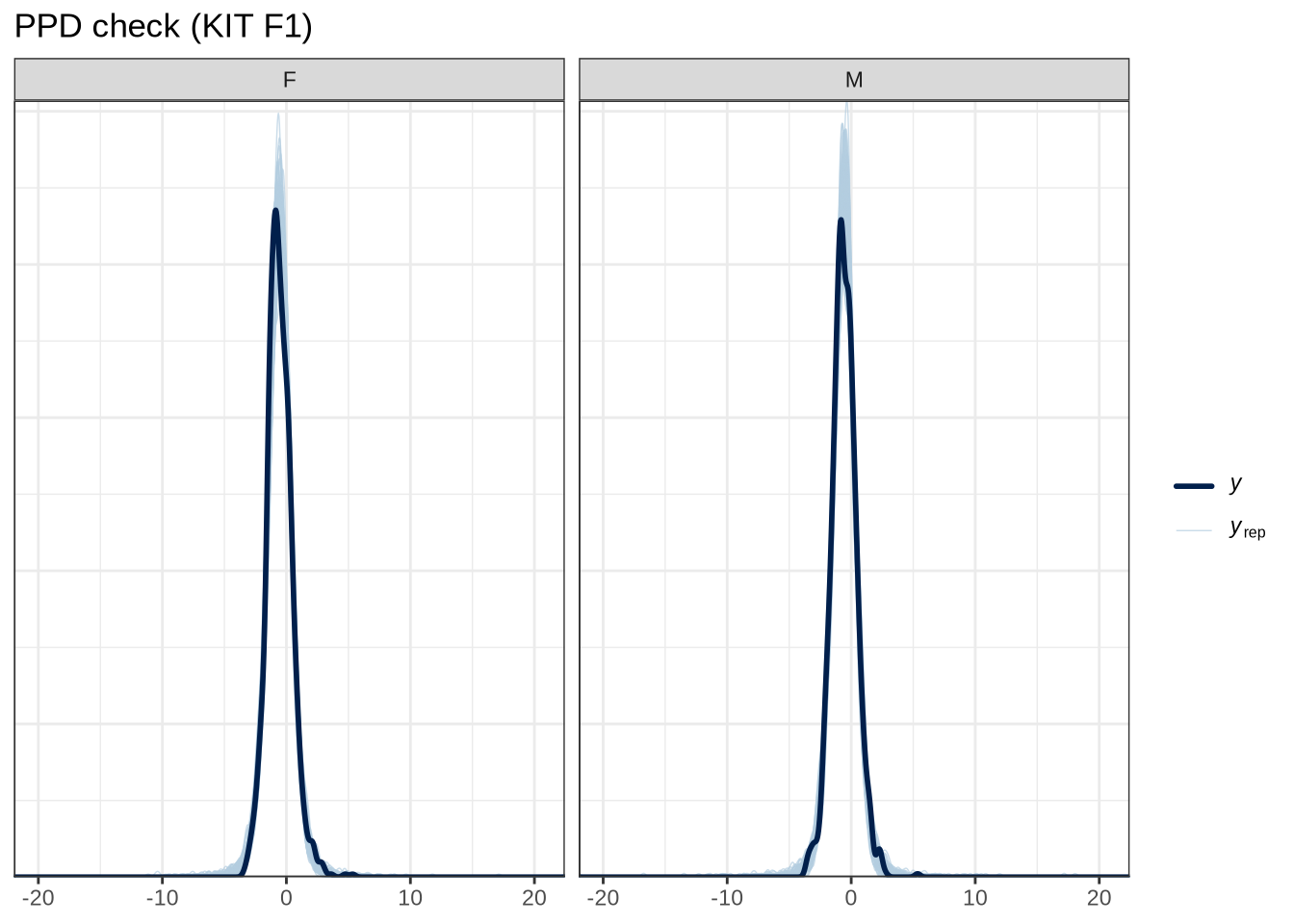
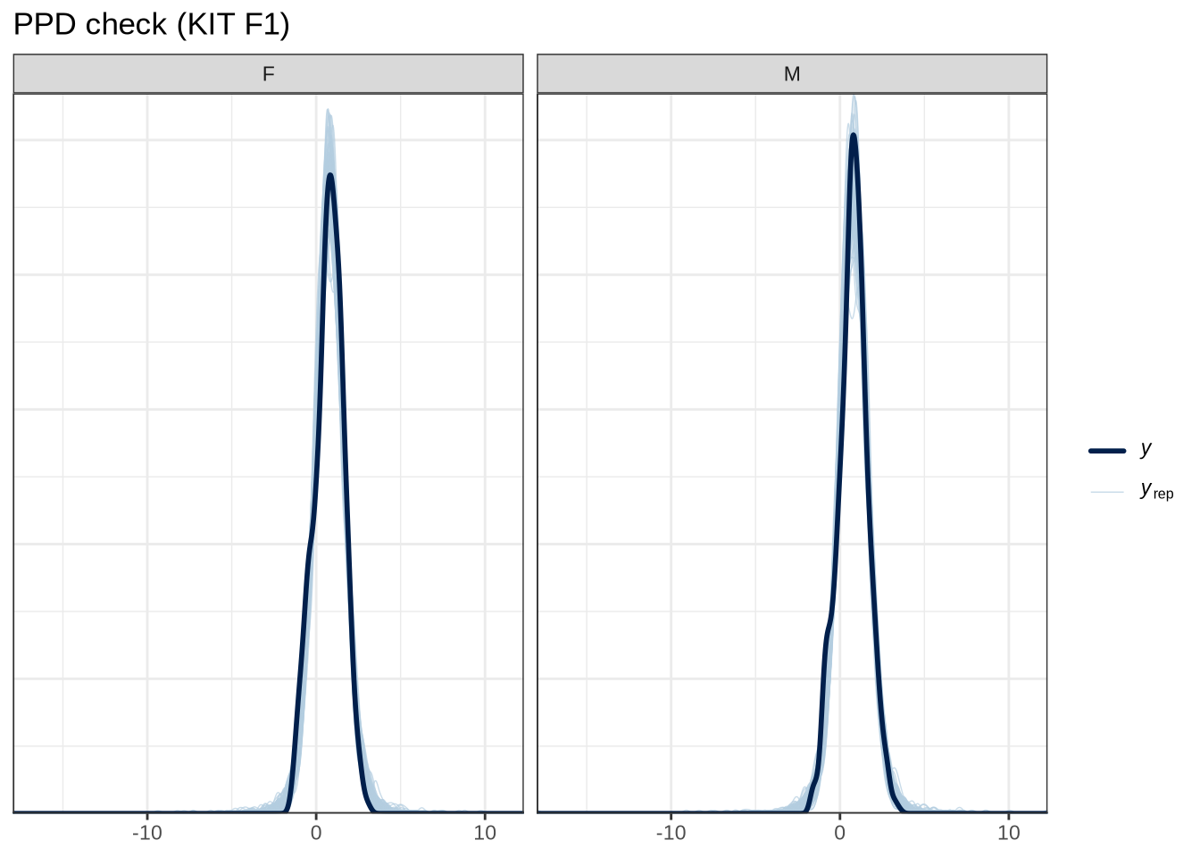
pp_check(kit_f1_fit, type="dens_overlay_grouped", group="gender", ndraws = 100) +
  labs(
    title = "PPD check (KIT F1)"
  )
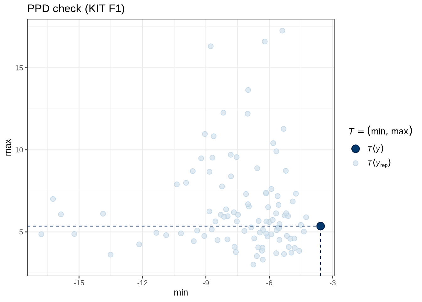
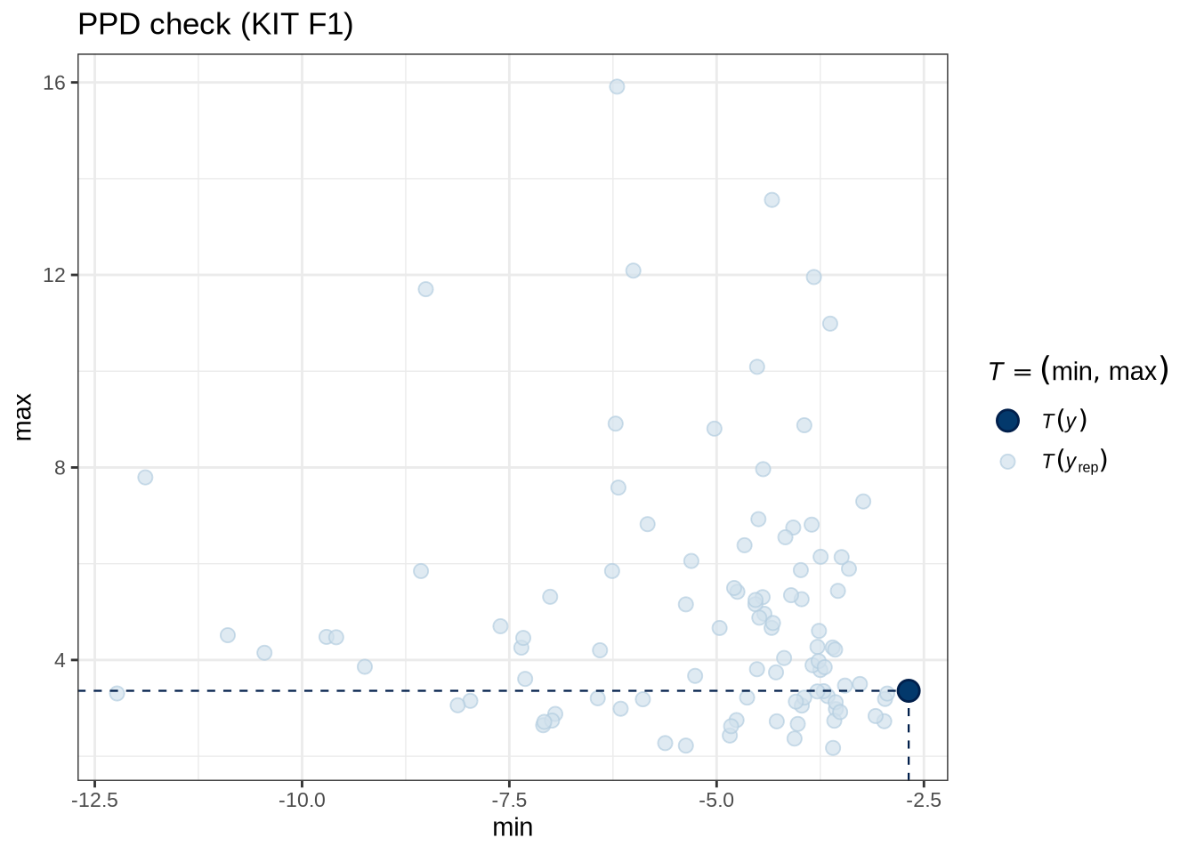
pp_check(kit_f1_fit, type = "stat_2d", stat = c("min", "max"), ndraws = 100) +
  labs(
    title = "PPD check (KIT F1)"
  )
model_plots(kit_f1_fit) +
  plot_annotation(title = "KIT F1")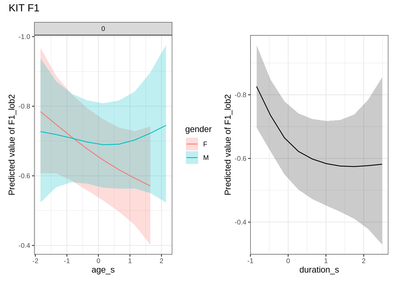
Female preschoolers look like they are lowering [kit] in the vowel space.
kit_f1_preds <- estimate_relation(
    kit_f1_fit,
    by = list(
      age_s = seq(min_age_s, max_age_s, length = 50),
      gender = c("F", "M"),
      duration_s = 0
    ),
    predict="link",
    ci = c(0.9, 0.7)
  )
Let’s see if the lowering patterns shows up in the data, viewed longitudinally.
diff_check(kit_f1_fit, kit_f1_data) %>%
  diff_plot()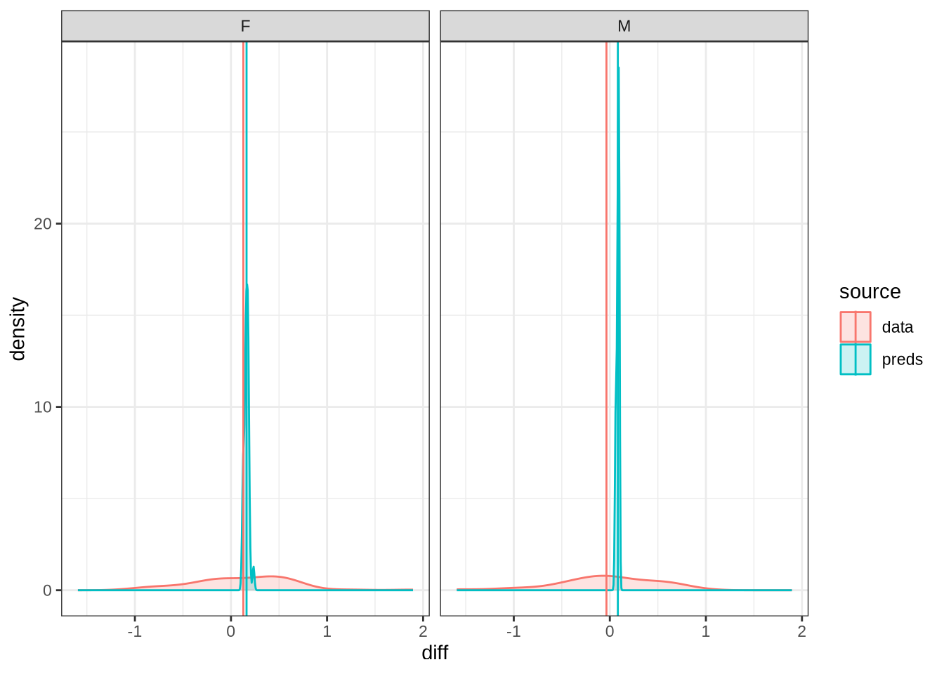
Figure 21 is a little chaotic. We see that a lot of the predictions are crushed into a a tight range in our predictions. We’ve divided by gender as the pattern identified only seems clear in the female speakers. In both cases, the shifts between sessions are in the positive direction, although the distribution sits very close to zero! In any case, what we are looking for here is significant incompatibility between the distribution of shifts between collection points and the corresponding model predictions.
kit_f1_10 <- ten_month_preds(kit_f1_fit, sample_points)
kit_f1_10 %>%
  ggplot(
    aes(
      x = diff,
      colour = gender,
      fill = gender
    )
  ) +
  geom_density(linewidth = 1, alpha = 0.2) +
  geom_vline(xintercept = 0, linetype = "dashed")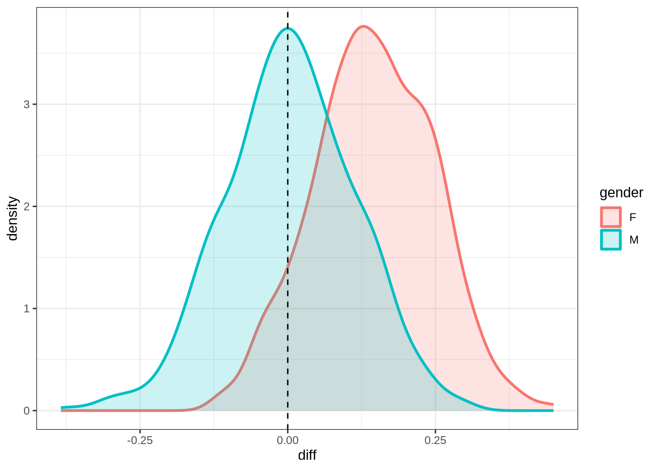
4.1.2.0.4 F2
kit_f2_data <- f2 |>
  filter(
    vowel == "KIT"
  ) |>
  mutate(
    w_s = interaction(word, stressed),
    p_c = interaction(participant, collect)
  ) %>%
  droplevels()


summary(kit_f2_data)
participant collect age_s gender word
Length:1801 Min. :1.00 Min. :-1.83828 F:952 his : 205
Class :character 1st Qu.:2.00 1st Qu.:-0.84298 M:849 him : 193
Mode :character Median :3.00 Median : 0.15231 it : 115
Mean :2.79 Mean : 0.05726 bridge : 89
3rd Qu.:4.00 3rd Qu.: 0.89878 the : 88
Max. :4.00 Max. : 2.64055 baby : 62
(Other):1049
vowel stressed stopword F2_lob2
KIT:1801 Mode :logical Mode :logical Min. :-1.6722
FALSE:623 FALSE:1007 1st Qu.: 0.2130
TRUE :1178 TRUE :794 Median : 0.7956
Mean : 0.7546
3rd Qu.: 1.3374
Max. : 3.5166
duration_s age w_s p_c
Min. :-0.83729 Min. :47.00 his.TRUE : 196 EC1402-Child.3: 35
1st Qu.:-0.58349 1st Qu.:51.00 him.TRUE : 178 EC0405-Child.2: 30
Median :-0.27489 Median :55.00 it.TRUE : 112 EC0918-Child.4: 28
Mean :-0.09937 Mean :54.62 the.TRUE : 88 EC0102-Child.4: 23
3rd Qu.: 0.17504 3rd Qu.:58.00 bridge.TRUE: 87 EC0901-Child.4: 23
Max. : 2.48745 Max. :65.00 baby.FALSE : 62 EC0501-Child.1: 21
(Other) :1078 (Other) :1641 kit_f2_fit <- brm(
F2_lob2 ~ gender + stopword +
s(age_s, by=gender, k = 5) +
s(duration_s, k = 5) +
(1 | w_s) +
(1 | p_c),
data = kit_f2_data,
family = student(),
prior = prior_t,
chains = 4,
cores = 4,
iter = 5000,
control = list(adapt_delta = 0.99),
)
write_rds(kit_f2_fit, here('models', 'kit_f2_fit_t.rds'), compress = "gz")kit_f2_fit <- read_rds(here('models', 'kit_f2_fit_t.rds'))summary(kit_f2_fit) Family: student
Links: mu = identity; sigma = identity; nu = identity
Formula: F2_lob2 ~ gender + stopword + s(age_s, by = gender, k = 5) + s(duration_s, k = 5) + (1 | w_s) + (1 | p_c)
Data: kit_f2_data (Number of observations: 1801)
Draws: 4 chains, each with iter = 5000; warmup = 2500; thin = 1;
total post-warmup draws = 10000
Smoothing Spline Hyperparameters:
Estimate Est.Error l-95% CI u-95% CI Rhat Bulk_ESS
sds(sage_sgenderF_1) 0.28 0.23 0.01 0.86 1.00 5038
sds(sage_sgenderM_1) 0.29 0.23 0.01 0.84 1.00 4539
sds(sduration_s_1) 0.29 0.22 0.01 0.84 1.00 4484
Tail_ESS
sds(sage_sgenderF_1) 4075
sds(sage_sgenderM_1) 4052
sds(sduration_s_1) 3831
Multilevel Hyperparameters:
~p_c (Number of levels: 201)
Estimate Est.Error l-95% CI u-95% CI Rhat Bulk_ESS Tail_ESS
sd(Intercept) 0.22 0.03 0.17 0.27 1.00 3372 5884
~w_s (Number of levels: 217)
Estimate Est.Error l-95% CI u-95% CI Rhat Bulk_ESS Tail_ESS
sd(Intercept) 0.51 0.05 0.43 0.61 1.00 2389 4583
Regression Coefficients:
Estimate Est.Error l-95% CI u-95% CI Rhat Bulk_ESS Tail_ESS
Intercept 0.93 0.06 0.81 1.04 1.00 3404 5999
genderM -0.01 0.05 -0.10 0.09 1.00 5933 7109
stopwordTRUE -0.17 0.14 -0.45 0.10 1.00 1505 2943
sage_s:genderF_1 0.06 0.49 -0.96 1.10 1.00 5623 5885
sage_s:genderM_1 -0.44 0.52 -1.43 0.70 1.00 5379 4907
sduration_s_1 0.93 0.45 -0.03 1.80 1.00 6095 5595
Further Distributional Parameters:
Estimate Est.Error l-95% CI u-95% CI Rhat Bulk_ESS Tail_ESS
sigma 0.59 0.02 0.54 0.63 1.00 4428 6909
nu 4.80 0.63 3.74 6.20 1.00 5636 6731
Draws were sampled using sampling(NUTS). For each parameter, Bulk_ESS
and Tail_ESS are effective sample size measures, and Rhat is the potential
scale reduction factor on split chains (at convergence, Rhat = 1).pp_check(kit_f2_fit, ndraws = 100) +
labs(
title = "PPD check (KIT F1)"
) 
pp_check(kit_f2_fit, type="dens_overlay_grouped", group="gender", ndraws = 100) +
  labs(
    title = "PPD check (KIT F1)"
  )
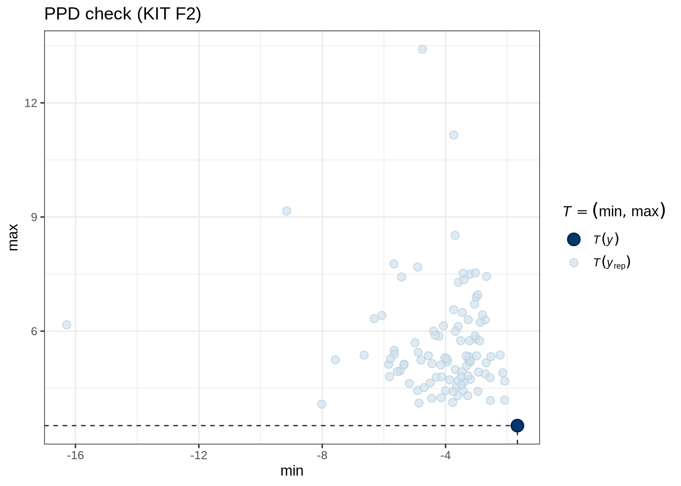
pp_check(kit_f2_fit, type = "stat_2d", stat = c("min", "max"), ndraws = 100) +
  labs(
    title = "PPD check (KIT F2)"
  )
model_plots(kit_f2_fit) +
  plot_annotation(title = "KIT F2")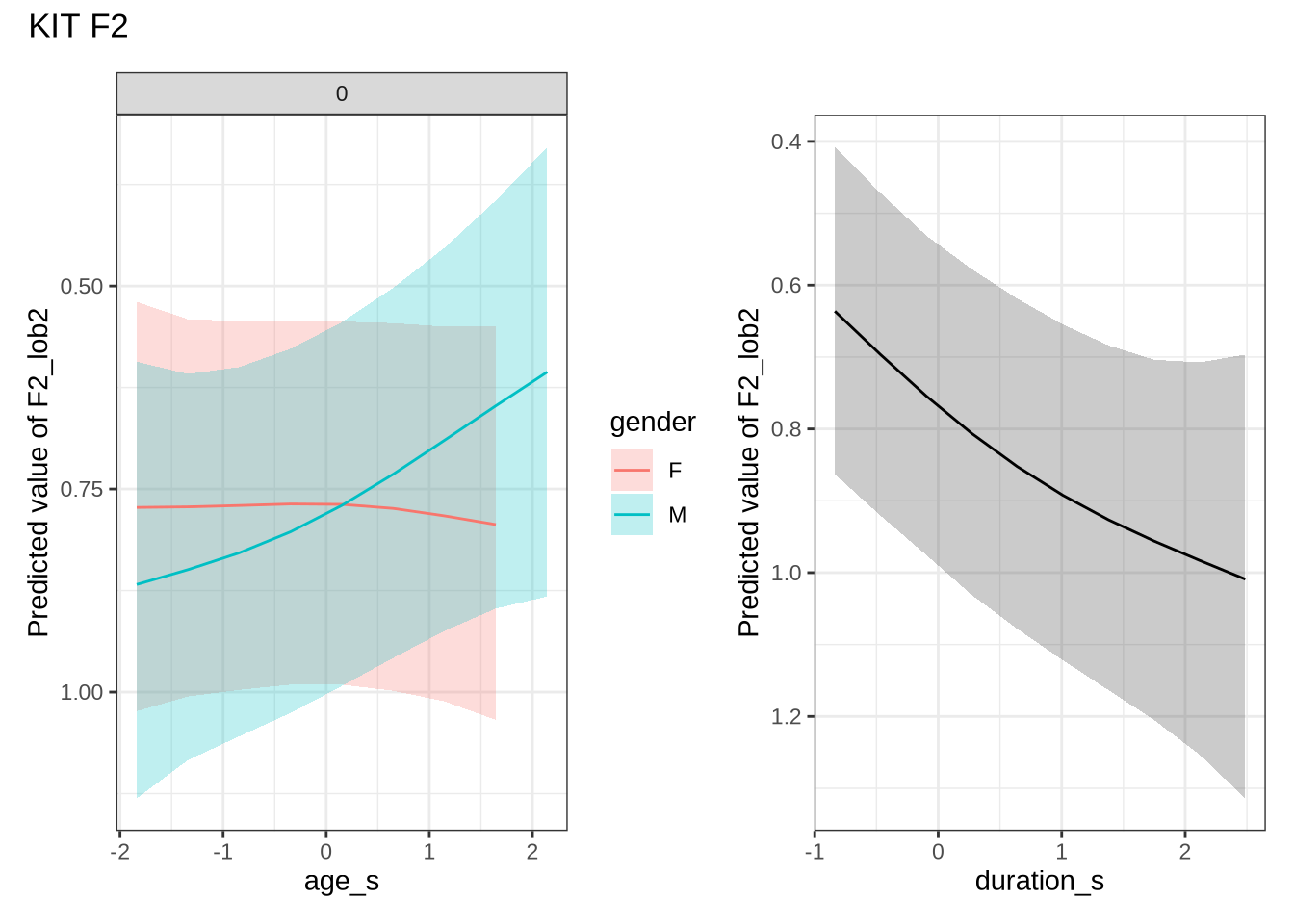
kit_f2_preds <- estimate_relation(
    kit_f2_fit,
    by = list(
      age_s = seq(min_age_s, max_age_s, length = 50),
      gender = c("F", "M"),
      duration_s = 0
    ),
    predict="link",
    ci = c(0.9, 0.7)
  )
There appears to be a backing in the vowel space for male preschoolers. Let’s see if this aligns with the data viewed longitudinally.
diff_check(kit_f2_fit, kit_f2_data) %>%
  diff_plot()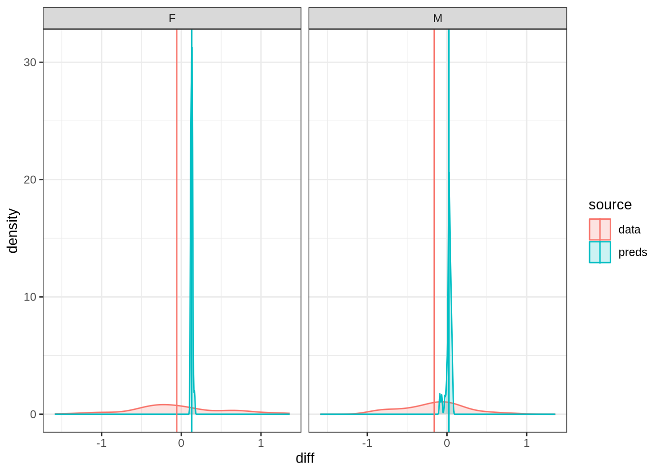
Figure 27 shows that our predictions are very tight and don’t particularly match the longitudinal data. For the male preschoolers we predict no change, but the longitudinal data suggests backing (as does our smooth). The female means appear on either side of zero for the predictions and the real longitudinal data. But we do not predict any significant change for female preschoolers in Figure 26.
kit_f2_10 <- ten_month_preds(kit_f2_fit, sample_points)
kit_f2_10 %>%
  ggplot(
    aes(
      x = diff,
      colour = gender,
      fill = gender
    )
  ) +
  geom_density(linewidth = 1, alpha = 0.2) +
  geom_vline(xintercept = 0, linetype = "dashed")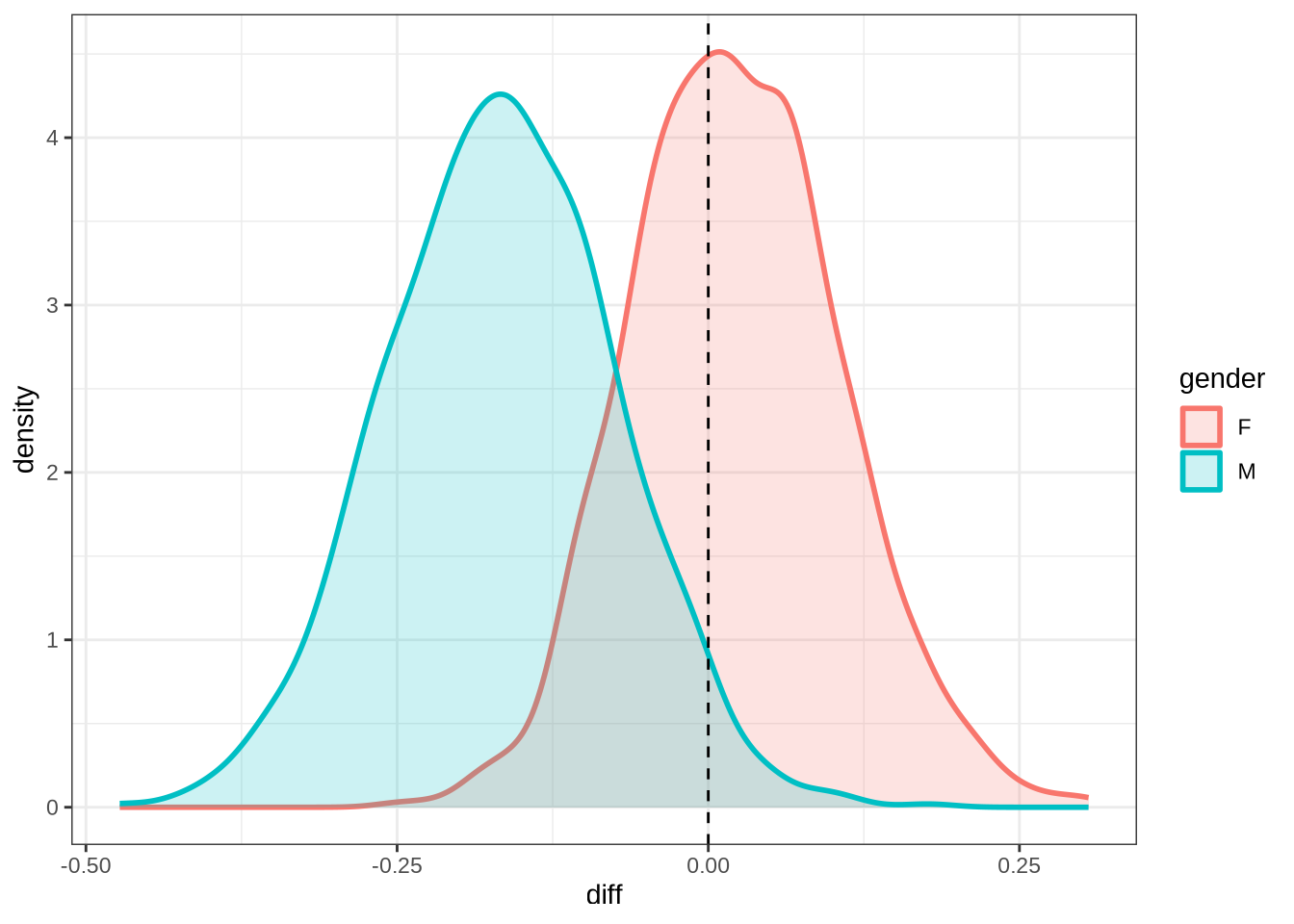
rm(
  kit_f1_fit,
  kit_f2_fit
)
4.1.2.0.5 F1
nurse_f1_data <- f1 |>
  filter(
    vowel == "NURSE"
  ) |>
  mutate(
    w_s = interaction(word, stressed),
    p_c = interaction(participant, collect)
  ) %>%
  droplevels()


summary(nurse_f1_data)
participant collect age_s gender word
Length:434 Min. :1.000 Min. :-1.8383 F:256 her :178
Class :character 1st Qu.:1.000 1st Qu.:-1.0918 M:178 bird : 85
Mode :character Median :2.000 Median :-0.3453 hurt : 71
Mean :2.302 Mean :-0.2697 work : 19
3rd Qu.:3.000 3rd Qu.: 0.4011 heard : 17
Max. :4.000 Max. : 2.6405 were : 15
(Other): 49
vowel stressed stopword F1_lob2
NURSE:434 Mode :logical Mode :logical Min. :-2.6838
FALSE:14 FALSE:241 1st Qu.:-0.8304
TRUE :420 TRUE :193 Median :-0.2094
Mean :-0.2098
3rd Qu.: 0.3456
Max. : 3.3603
duration_s age w_s p_c
Min. :-1.2577 Min. :47.0 her.TRUE :176 EC0501-Child.1: 13
1st Qu.:-0.7247 1st Qu.:50.0 bird.TRUE : 84 EC2308-Child.1: 12
Median :-0.2805 Median :53.0 hurt.TRUE : 68 EC0511-Child.2: 12
Mean :-0.1426 Mean :53.3 work.TRUE : 17 EC0524-Child.2: 11
3rd Qu.: 0.2909 3rd Qu.:56.0 heard.TRUE: 16 EC0421-Child.2: 10
Max. : 2.3844 Max. :65.0 were.TRUE : 14 EC0520-Child.2: 8
(Other) : 59 (Other) :368 nurse_f1_fit <- brm(
F1_lob2 ~ gender + stopword +
s(age_s, by=gender, k = 5) +
s(duration_s, k = 5) +
(1 | w_s) +
(1 | p_c),
data = nurse_f1_data,
family = student(),
prior = prior_t,
chains = 4,
cores = 4,
iter = 3000,
control = list(adapt_delta = 0.9),
)
write_rds(nurse_f1_fit, here('models', 'nurse_f1_fit_t.rds'), compress = "gz")nurse_f1_fit <- read_rds(here('models', 'nurse_f1_fit_t.rds'))summary(nurse_f1_fit) Family: student
Links: mu = identity; sigma = identity; nu = identity
Formula: F1_lob2 ~ gender + stopword + s(age_s, by = gender, k = 5) + s(duration_s, k = 5) + (1 | w_s) + (1 | p_c)
Data: nurse_f1_data (Number of observations: 434)
Draws: 4 chains, each with iter = 3000; warmup = 1500; thin = 1;
total post-warmup draws = 6000
Smoothing Spline Hyperparameters:
Estimate Est.Error l-95% CI u-95% CI Rhat Bulk_ESS
sds(sage_sgenderF_1) 0.35 0.27 0.02 1.00 1.00 3977
sds(sage_sgenderM_1) 0.37 0.28 0.02 1.06 1.00 3728
sds(sduration_s_1) 0.38 0.27 0.02 1.02 1.00 2555
Tail_ESS
sds(sage_sgenderF_1) 2790
sds(sage_sgenderM_1) 2729
sds(sduration_s_1) 2443
Multilevel Hyperparameters:
~p_c (Number of levels: 151)
Estimate Est.Error l-95% CI u-95% CI Rhat Bulk_ESS Tail_ESS
sd(Intercept) 0.40 0.06 0.28 0.53 1.00 1787 2795
~w_s (Number of levels: 34)
Estimate Est.Error l-95% CI u-95% CI Rhat Bulk_ESS Tail_ESS
sd(Intercept) 0.21 0.11 0.03 0.46 1.00 1346 1419
Regression Coefficients:
Estimate Est.Error l-95% CI u-95% CI Rhat Bulk_ESS Tail_ESS
Intercept -0.25 0.11 -0.46 -0.03 1.00 3475 3996
genderM 0.01 0.11 -0.20 0.22 1.00 3136 3982
stopwordTRUE 0.08 0.19 -0.30 0.49 1.00 2747 2731
sage_s:genderF_1 0.59 0.80 -1.02 2.14 1.00 3350 3815
sage_s:genderM_1 -0.56 0.83 -2.24 1.10 1.00 3597 3436
sduration_s_1 0.41 0.74 -0.80 2.13 1.00 2908 3022
Further Distributional Parameters:
Estimate Est.Error l-95% CI u-95% CI Rhat Bulk_ESS Tail_ESS
sigma 0.59 0.04 0.51 0.67 1.00 2691 3925
nu 3.45 0.60 2.45 4.81 1.00 4077 4447
Draws were sampled using sampling(NUTS). For each parameter, Bulk_ESS
and Tail_ESS are effective sample size measures, and Rhat is the potential
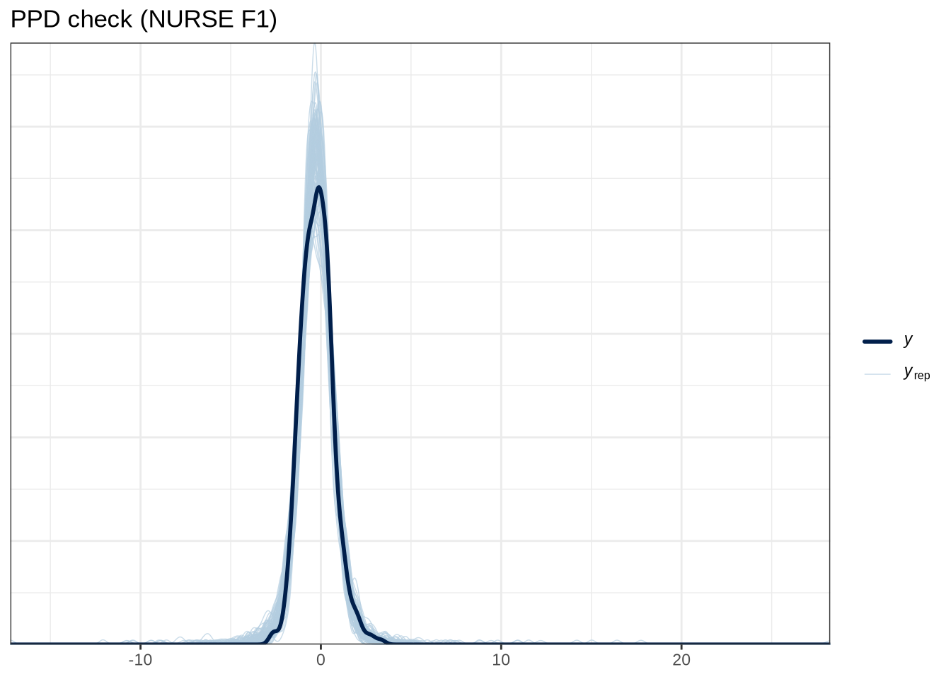
scale reduction factor on split chains (at convergence, Rhat = 1).pp_check(nurse_f1_fit, ndraws = 100) +
labs(
title = "PPD check (NURSE F1)"
) 
pp_check(nurse_f1_fit, type = "stat_2d", stat = c("min", "max"), ndraws = 100) +
  labs(
    title = "PPD check (KIT F1)"
  )
model_plots(nurse_f1_fit) +
  plot_annotation(title = "NURSE F1")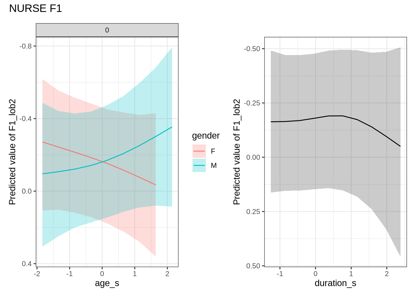
nurse_f1_preds <- estimate_relation(
    nurse_f1_fit,
    by = list(
      age_s = seq(min_age_s, max_age_s, length = 50),
      gender = c("F", "M"),
      duration_s = 0
    ),
    predict="link",
    ci = c(0.9, 0.7)
)diff_check(nurse_f1_fit, nurse_f1_data) %>%
diff_plot()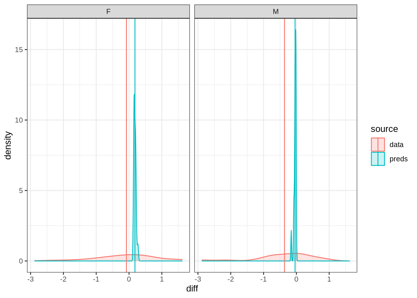
Out models predict some change over time for male preschoolers which, when the data is view longitudinally, looks even more extreme. We do not make a big deal of this, given the wide error bars on our models.
nurse_f1_10 <- ten_month_preds(nurse_f1_fit, sample_points)
nurse_f1_10 %>%
  ggplot(
    aes(
      x = diff,
      colour = gender,
      fill = gender
    )
  ) +
  geom_density(linewidth = 1, alpha = 0.2) +
  geom_vline(xintercept = 0, linetype = "dashed")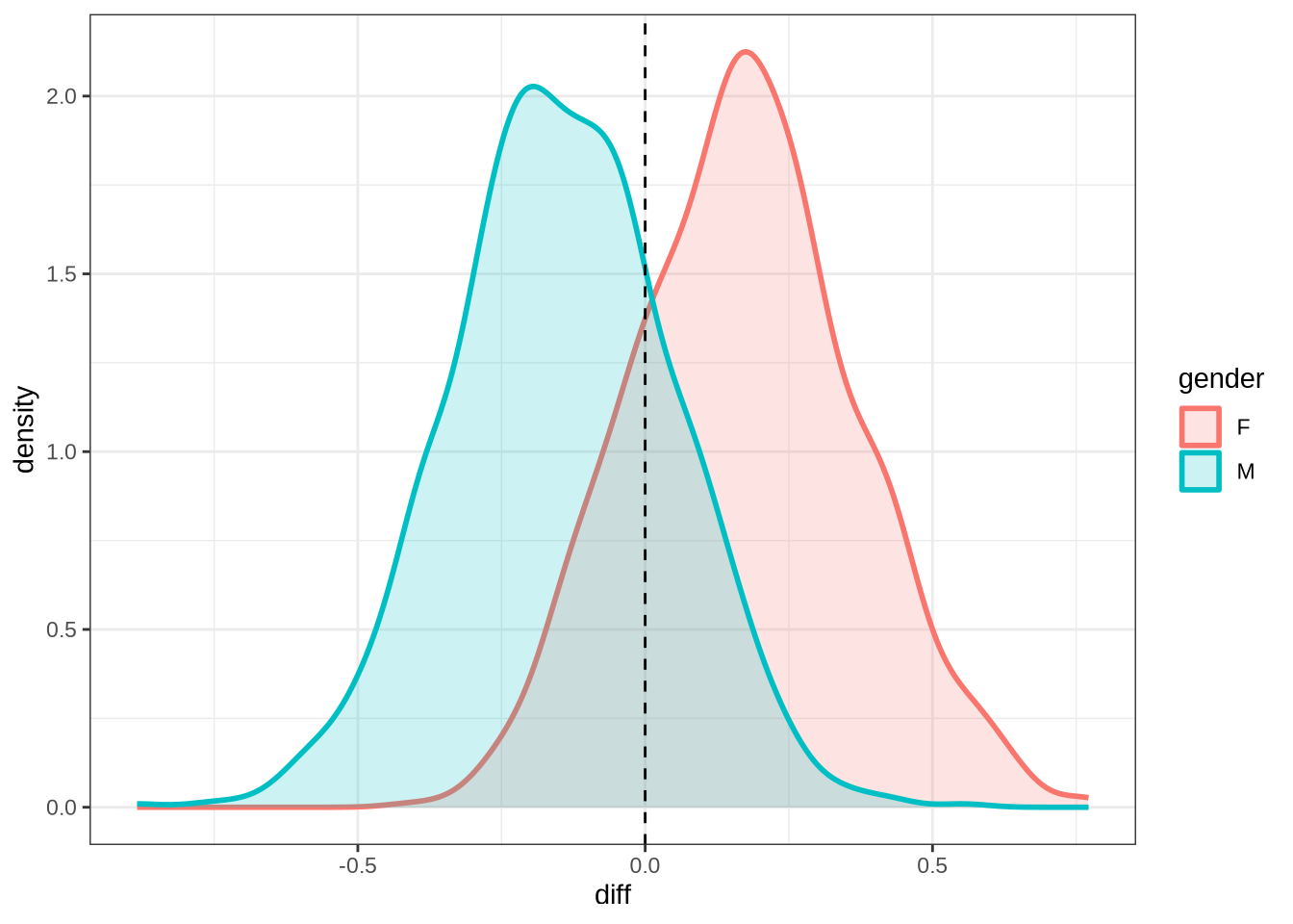
4.1.2.0.6 F2
nurse_f2_data <- f2 |>
  filter(
    vowel == "NURSE"
  ) |>
  mutate(
    w_s = interaction(word, stressed),
    p_c = interaction(participant, collect)
  ) %>%
  droplevels()


summary(nurse_f2_data)
participant collect age_s gender word
Length:435 Min. :1.000 Min. :-1.8383 F:252 her :182
Class :character 1st Qu.:1.000 1st Qu.:-1.0918 M:183 bird : 83
Mode :character Median :2.000 Median :-0.3453 hurt : 73
Mean :2.297 Mean :-0.2658 work : 18
3rd Qu.:3.000 3rd Qu.: 0.4011 were : 16
Max. :4.000 Max. : 2.6405 heard : 15
(Other): 48
vowel stressed stopword F2_lob2
NURSE:435 Mode :logical Mode :logical Min. :-1.8423
FALSE:13 FALSE:237 1st Qu.:-0.6160
TRUE :422 TRUE :198 Median : 0.0486
Mean :-0.0417
3rd Qu.: 0.5324
Max. : 1.6210
duration_s age w_s p_c
Min. :-1.2577 Min. :47.00 her.TRUE :180 EC0501-Child.1: 12
1st Qu.:-0.7247 1st Qu.:50.00 bird.TRUE : 82 EC2308-Child.1: 12
Median :-0.2805 Median :53.00 hurt.TRUE : 70 EC0511-Child.2: 12
Mean :-0.1366 Mean :53.32 work.TRUE : 16 EC0524-Child.2: 11
3rd Qu.: 0.2956 3rd Qu.:56.00 were.TRUE : 15 EC0421-Child.2: 10
Max. : 2.3844 Max. :65.00 heard.TRUE: 14 EC0520-Child.2: 8
(Other) : 58 (Other) :370 nurse_f2_fit <- brm(
F2_lob2 ~ gender + stopword +
s(age_s, by=gender, k = 5) +
s(duration_s, k = 5) +
(1 | w_s) +
(1 | p_c),
data = nurse_f2_data,
family = student(),
prior = prior_t,
chains = 4,
cores = 4,
iter = 4000,
control = list(adapt_delta = 0.9),
)
write_rds(nurse_f2_fit, here('models', 'nurse_f2_fit_t.rds'), compress = "gz")nurse_f2_fit <- read_rds(here('models', 'nurse_f2_fit_t.rds'))summary(nurse_f2_fit) Family: student
Links: mu = identity; sigma = identity; nu = identity
Formula: F2_lob2 ~ gender + stopword + s(age_s, by = gender, k = 5) + s(duration_s, k = 5) + (1 | w_s) + (1 | p_c)
Data: nurse_f2_data (Number of observations: 435)
Draws: 4 chains, each with iter = 4000; warmup = 2000; thin = 1;
total post-warmup draws = 8000
Smoothing Spline Hyperparameters:
Estimate Est.Error l-95% CI u-95% CI Rhat Bulk_ESS
sds(sage_sgenderF_1) 0.35 0.26 0.02 0.98 1.00 3987
sds(sage_sgenderM_1) 0.36 0.27 0.01 1.02 1.00 4195
sds(sduration_s_1) 0.28 0.23 0.01 0.83 1.00 4464
Tail_ESS
sds(sage_sgenderF_1) 3517
sds(sage_sgenderM_1) 3867
sds(sduration_s_1) 4468
Multilevel Hyperparameters:
~p_c (Number of levels: 153)
Estimate Est.Error l-95% CI u-95% CI Rhat Bulk_ESS Tail_ESS
sd(Intercept) 0.45 0.04 0.37 0.54 1.00 2114 3622
~w_s (Number of levels: 33)
Estimate Est.Error l-95% CI u-95% CI Rhat Bulk_ESS Tail_ESS
sd(Intercept) 0.25 0.07 0.12 0.41 1.00 2651 3998
Regression Coefficients:
Estimate Est.Error l-95% CI u-95% CI Rhat Bulk_ESS Tail_ESS
Intercept 0.10 0.10 -0.10 0.30 1.00 3921 4694
genderM -0.09 0.10 -0.30 0.10 1.00 3064 3867
stopwordTRUE -0.48 0.20 -0.89 -0.09 1.00 3396 4053
sage_s:genderF_1 -0.65 0.79 -2.21 1.04 1.00 3975 4155
sage_s:genderM_1 -0.28 0.79 -1.88 1.30 1.00 3896 4324
sduration_s_1 -0.00 0.52 -0.97 1.17 1.00 5300 4647
Further Distributional Parameters:
Estimate Est.Error l-95% CI u-95% CI Rhat Bulk_ESS Tail_ESS
sigma 0.44 0.03 0.38 0.50 1.00 3171 4456
nu 3.77 0.73 2.57 5.40 1.00 4656 5120
Draws were sampled using sampling(NUTS). For each parameter, Bulk_ESS
and Tail_ESS are effective sample size measures, and Rhat is the potential
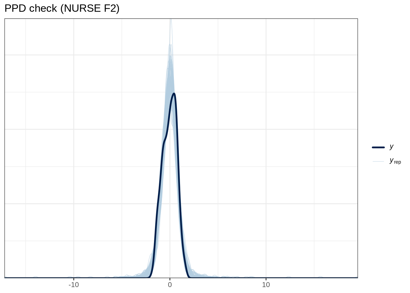
scale reduction factor on split chains (at convergence, Rhat = 1).pp_check(nurse_f2_fit, ndraws = 100) +
labs(
title = "PPD check (NURSE F2)"
) 
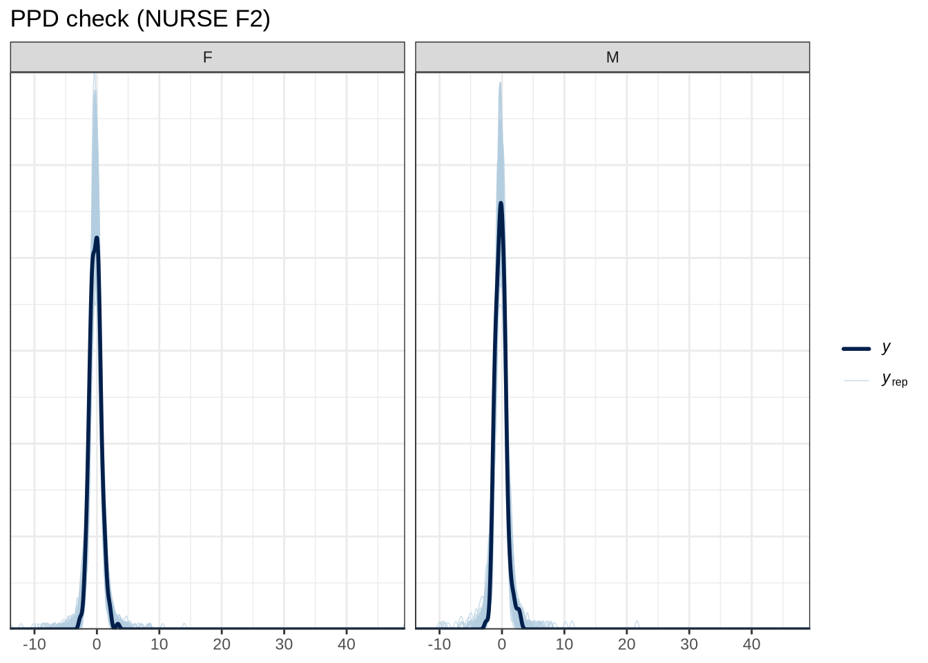
pp_check(nurse_f1_fit, type="dens_overlay_grouped", group="gender", ndraws = 100) +
  labs(
    title = "PPD check (NURSE F2)"
  )
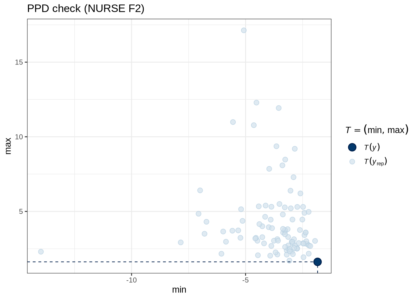
pp_check(nurse_f2_fit, type = "stat_2d", stat = c("min", "max"), ndraws = 100) +
  labs(
    title = "PPD check (NURSE F2)"
  )
model_plots(nurse_f2_fit) +
  plot_annotation(title = "NURSE F2")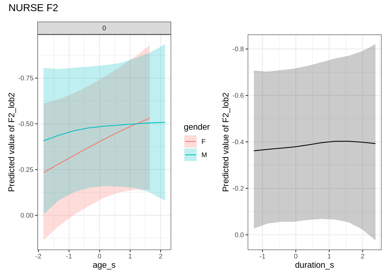
nurse_f2_preds <- estimate_relation(
    nurse_f2_fit,
    by = list(
      age_s = seq(min_age_s, max_age_s, length = 50),
      gender = c("F", "M"),
      duration_s = 0
    ),
    predict="link",
    ci = c(0.9, 0.7)
)diff_check(nurse_f2_fit, nurse_f2_data) %>%
diff_plot()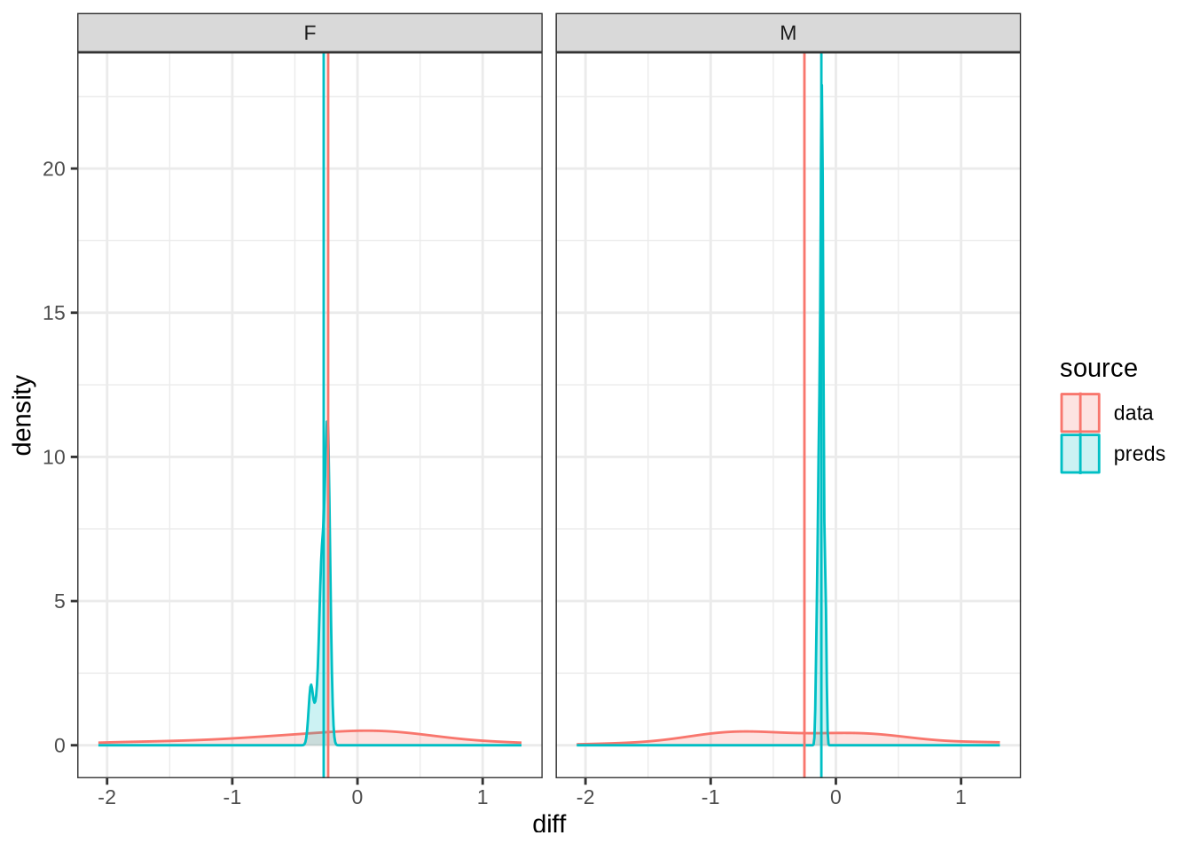
We won’t be taking nurse seriously in the paper. Nonetheless, it is interesting to see how narrow the distribution of predicted differencess between sessions is in our models compared to the real range of variation between sessions (which can just be seen at the bottom of the plot).
nurse_f2_10 <- ten_month_preds(nurse_f2_fit, sample_points)
nurse_f2_10 %>%
  ggplot(
    aes(
      x = diff,
      colour = gender,
      fill = gender
    )
  ) +
  geom_density(linewidth = 1, alpha = 0.2) +
  geom_vline(xintercept = 0, linetype = "dashed")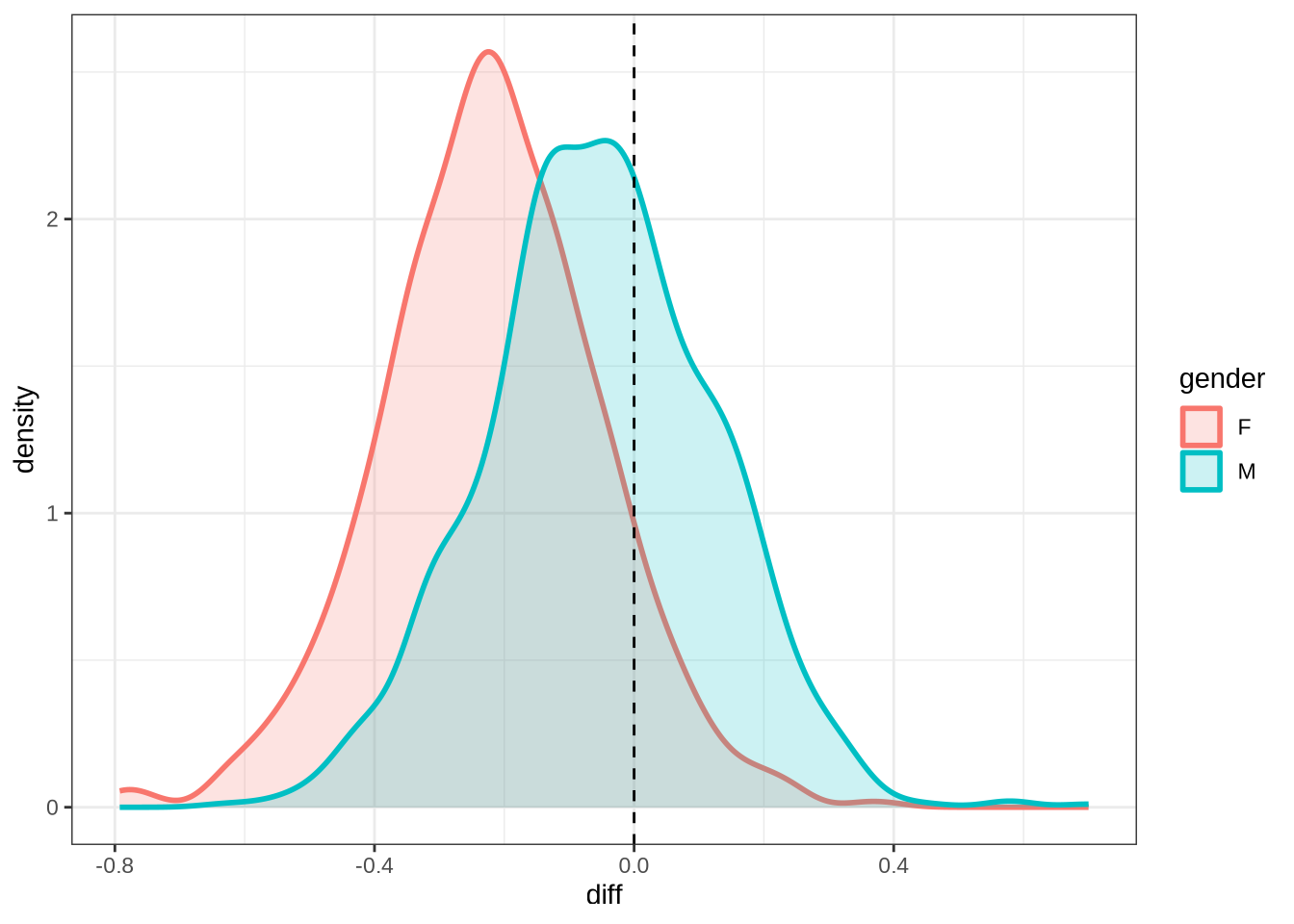
rm(
  nurse_f1_fit,
  nurse_f2_fit
)
4.1.2.0.7 F1
trap_f1_data <- f1 |>
  filter(
    vowel == "TRAP"
  ) |>
  mutate(
    w_s = interaction(word, stressed),
    p_c = interaction(participant, collect)
  ) %>%
  droplevels()


summary(trap_f1_data)
participant collect age_s gender word
Length:958 Min. :1.000 Min. :-1.8383 F:547 and :390
Class :character 1st Qu.:2.000 1st Qu.:-0.5942 M:411 nana :146
Mode :character Median :3.000 Median : 0.1523 that : 92
Mean :2.881 Mean : 0.0827 back : 62
3rd Qu.:4.000 3rd Qu.: 0.8988 grandma: 28
Max. :4.000 Max. : 2.6405 that's : 24
(Other):216
vowel stressed stopword F1_lob2
TRAP:958 Mode :logical Mode :logical Min. :-4.5669
FALSE:42 FALSE:370 1st Qu.:-0.1958
TRUE :916 TRUE :588 Median : 0.7648
Mean : 0.8560
3rd Qu.: 1.7636
Max. : 7.5250
duration_s age w_s p_c
Min. :-0.79502 Min. :47.00 and.TRUE :373 EC0405-Child.2: 20
1st Qu.:-0.48804 1st Qu.:52.00 nana.TRUE :139 EC0105-Child.2: 18
Median :-0.25780 Median :55.00 that.TRUE : 88 EC2432-Child.3: 18
Mean :-0.11420 Mean :54.72 back.TRUE : 61 EC0118-Child.4: 18
3rd Qu.: 0.04918 3rd Qu.:58.00 grandma.TRUE: 24 EC1424-Child.3: 14
Max. : 2.42830 Max. :65.00 that's.TRUE : 23 EC0607-Child.4: 14
(Other) :250 (Other) :856 trap_f1_fit <- brm(
F1_lob2 ~ gender + stopword +
s(age_s, by=gender, k = 5) +
s(duration_s, k = 5) +
(1 | w_s) +
(1 | p_c),
data = trap_f1_data,
family = student(),
prior = prior_t,
chains = 4,
cores = 4,
iter = 3000,
control = list(adapt_delta = 0.9),
)
write_rds(trap_f1_fit, here('models', 'trap_f1_fit_t.rds'), compress = "gz")trap_f1_fit <- read_rds(here('models', 'trap_f1_fit_t.rds'))summary(trap_f1_fit) Family: student
Links: mu = identity; sigma = identity; nu = identity
Formula: F1_lob2 ~ gender + stopword + s(age_s, by = gender, k = 5) + s(duration_s, k = 5) + (1 | w_s) + (1 | p_c)
Data: trap_f1_data (Number of observations: 958)
Draws: 4 chains, each with iter = 3000; warmup = 1500; thin = 1;
total post-warmup draws = 6000
Smoothing Spline Hyperparameters:
Estimate Est.Error l-95% CI u-95% CI Rhat Bulk_ESS
sds(sage_sgenderF_1) 0.37 0.27 0.01 1.00 1.00 4066
sds(sage_sgenderM_1) 0.34 0.26 0.01 0.99 1.00 5001
sds(sduration_s_1) 0.38 0.28 0.02 1.07 1.00 4556
Tail_ESS
sds(sage_sgenderF_1) 3379
sds(sage_sgenderM_1) 3616
sds(sduration_s_1) 3588
Multilevel Hyperparameters:
~p_c (Number of levels: 185)
Estimate Est.Error l-95% CI u-95% CI Rhat Bulk_ESS Tail_ESS
sd(Intercept) 0.33 0.08 0.16 0.47 1.00 1640 1738
~w_s (Number of levels: 73)
Estimate Est.Error l-95% CI u-95% CI Rhat Bulk_ESS Tail_ESS
sd(Intercept) 0.45 0.10 0.28 0.68 1.00 3222 4378
Regression Coefficients:
Estimate Est.Error l-95% CI u-95% CI Rhat Bulk_ESS Tail_ESS
Intercept 0.92 0.14 0.64 1.20 1.00 6614 4711
genderM 0.05 0.11 -0.17 0.26 1.00 9091 4760
stopwordTRUE 0.10 0.21 -0.33 0.52 1.00 3773 4059
sage_s:genderF_1 0.88 0.77 -0.75 2.37 1.00 5902 4026
sage_s:genderM_1 -0.59 0.77 -2.16 0.89 1.00 6847 4584
sduration_s_1 0.38 0.83 -1.25 2.09 1.00 7689 4757
Further Distributional Parameters:
Estimate Est.Error l-95% CI u-95% CI Rhat Bulk_ESS Tail_ESS
sigma 1.13 0.05 1.03 1.22 1.00 3704 4571
nu 4.43 0.63 3.34 5.81 1.00 5712 4954
Draws were sampled using sampling(NUTS). For each parameter, Bulk_ESS
and Tail_ESS are effective sample size measures, and Rhat is the potential
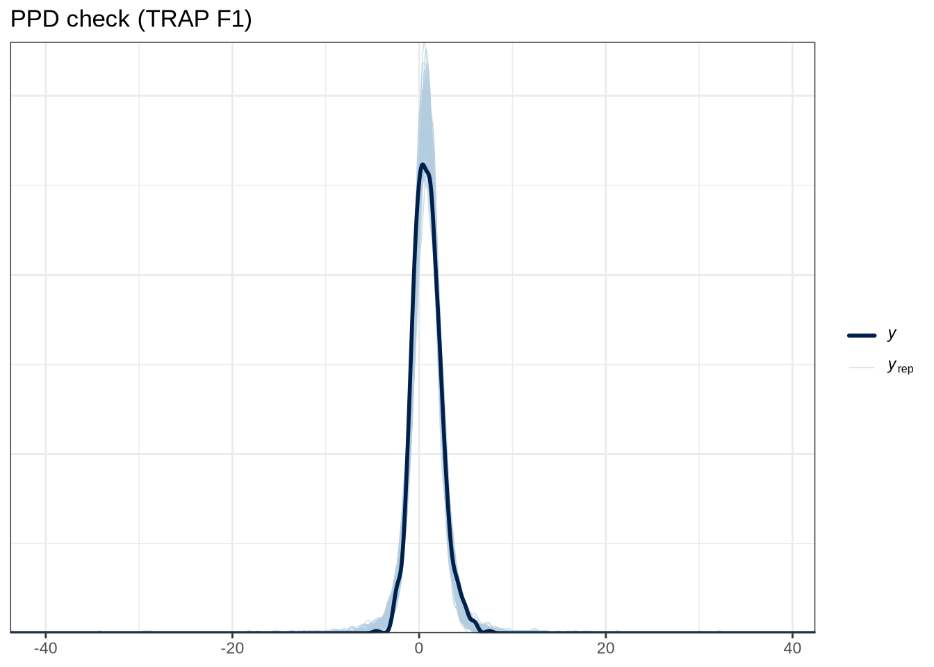
scale reduction factor on split chains (at convergence, Rhat = 1).pp_check(trap_f1_fit, ndraws = 100) +
labs(
title = "PPD check (TRAP F1)"
) 
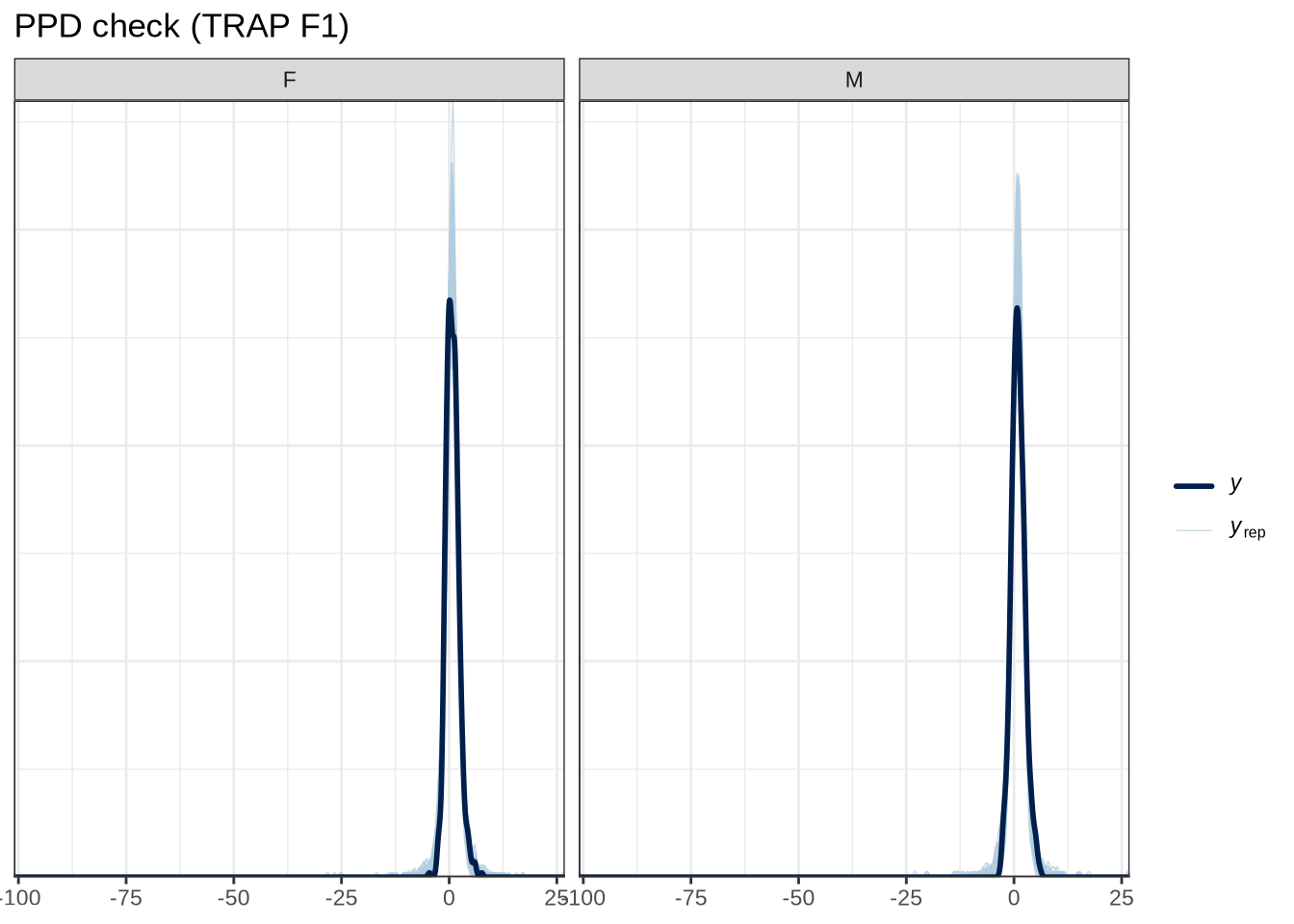
pp_check(trap_f1_fit, type="dens_overlay_grouped", group="gender", ndraws = 100) +
  labs(
    title = "PPD check (TRAP F1)"
  )
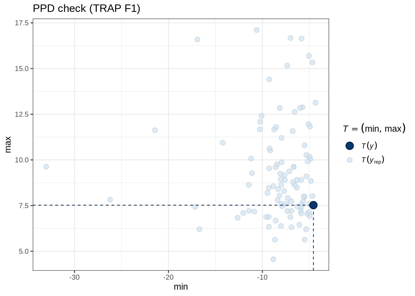
pp_check(trap_f1_fit, type = "stat_2d", stat = c("min", "max"), ndraws = 100) +
  labs(
    title = "PPD check (TRAP F1)"
  )
model_plots(trap_f1_fit) +
  plot_annotation(title = "TRAP F1")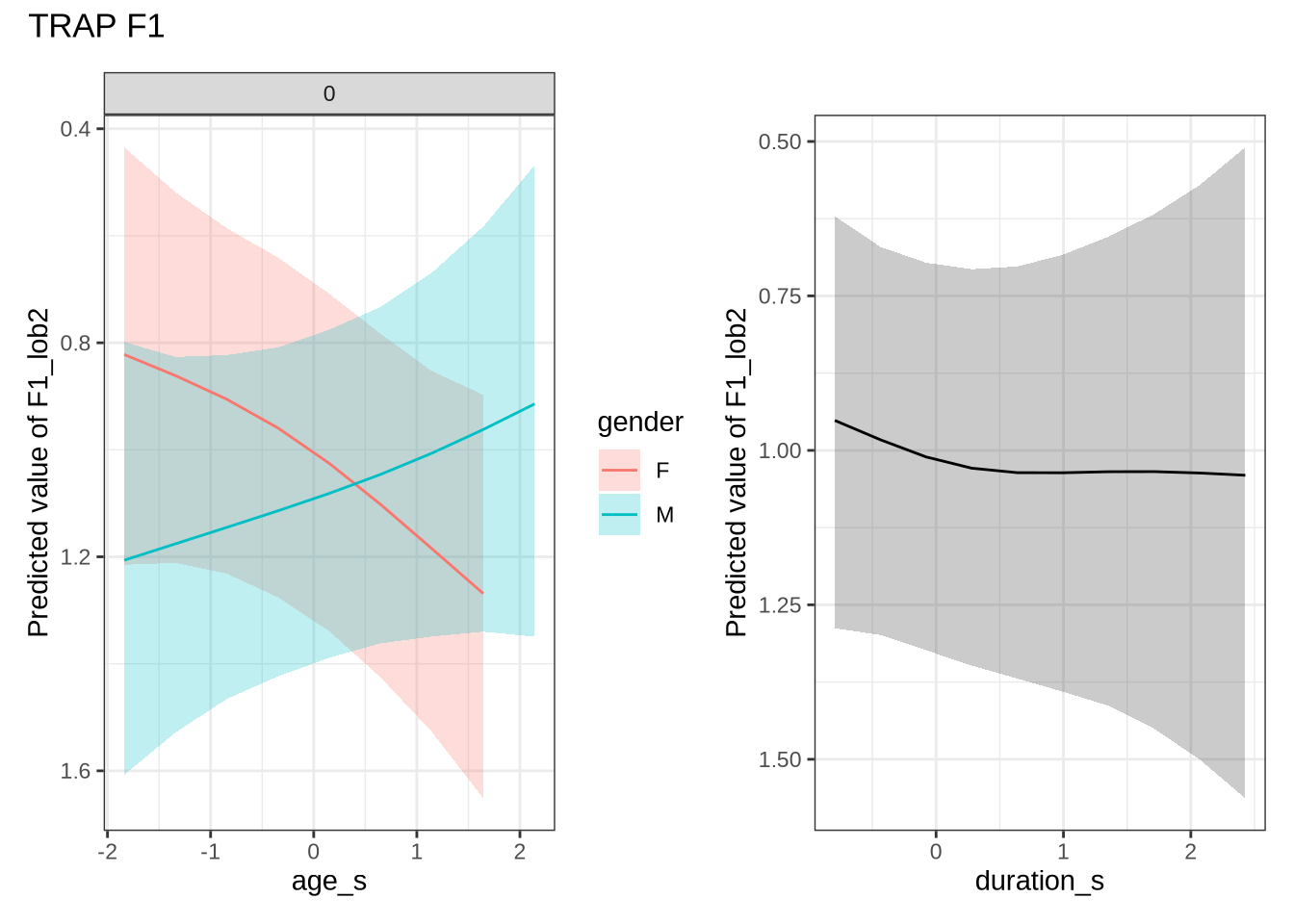
trap_f1_preds <- estimate_relation(
    trap_f1_fit,
    by = list(
      age_s = seq(min_age_s, max_age_s, length = 50),
      gender = c("F", "M"),
      duration_s = 0
    ),
    predict="link",
    ci = c(0.9, 0.7)
)diff_check(trap_f1_fit, trap_f1_data) %>%
diff_plot()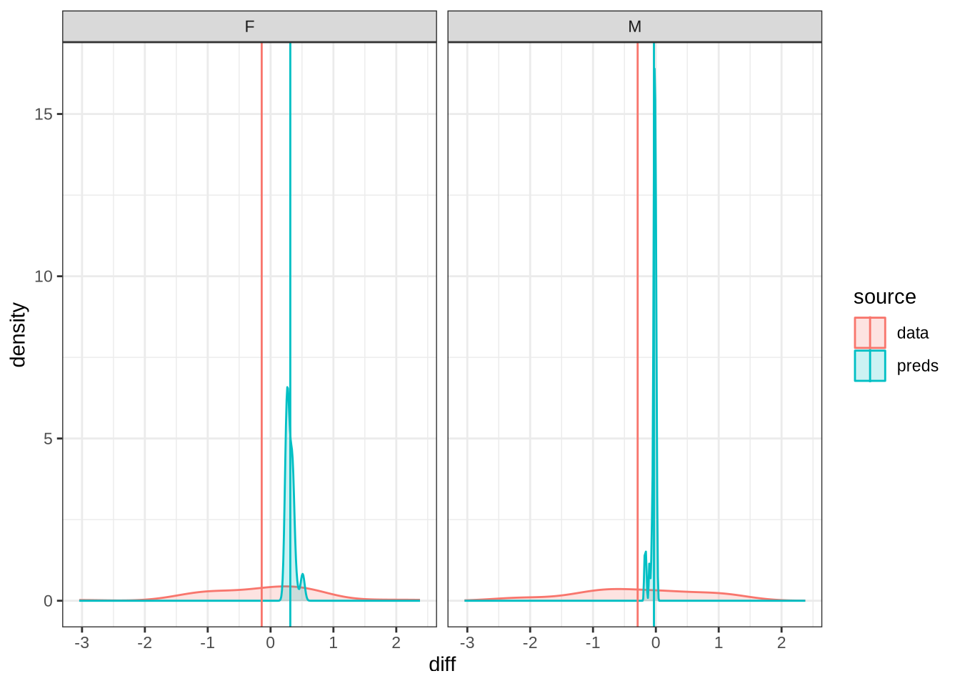
trap_f1_10 <- ten_month_preds(trap_f1_fit, sample_points)
trap_f1_10 %>%
  ggplot(
    aes(
      x = diff,
      colour = gender,
      fill = gender
    )
  ) +
  geom_density(linewidth = 1, alpha = 0.2) +
  geom_vline(xintercept = 0, linetype = "dashed")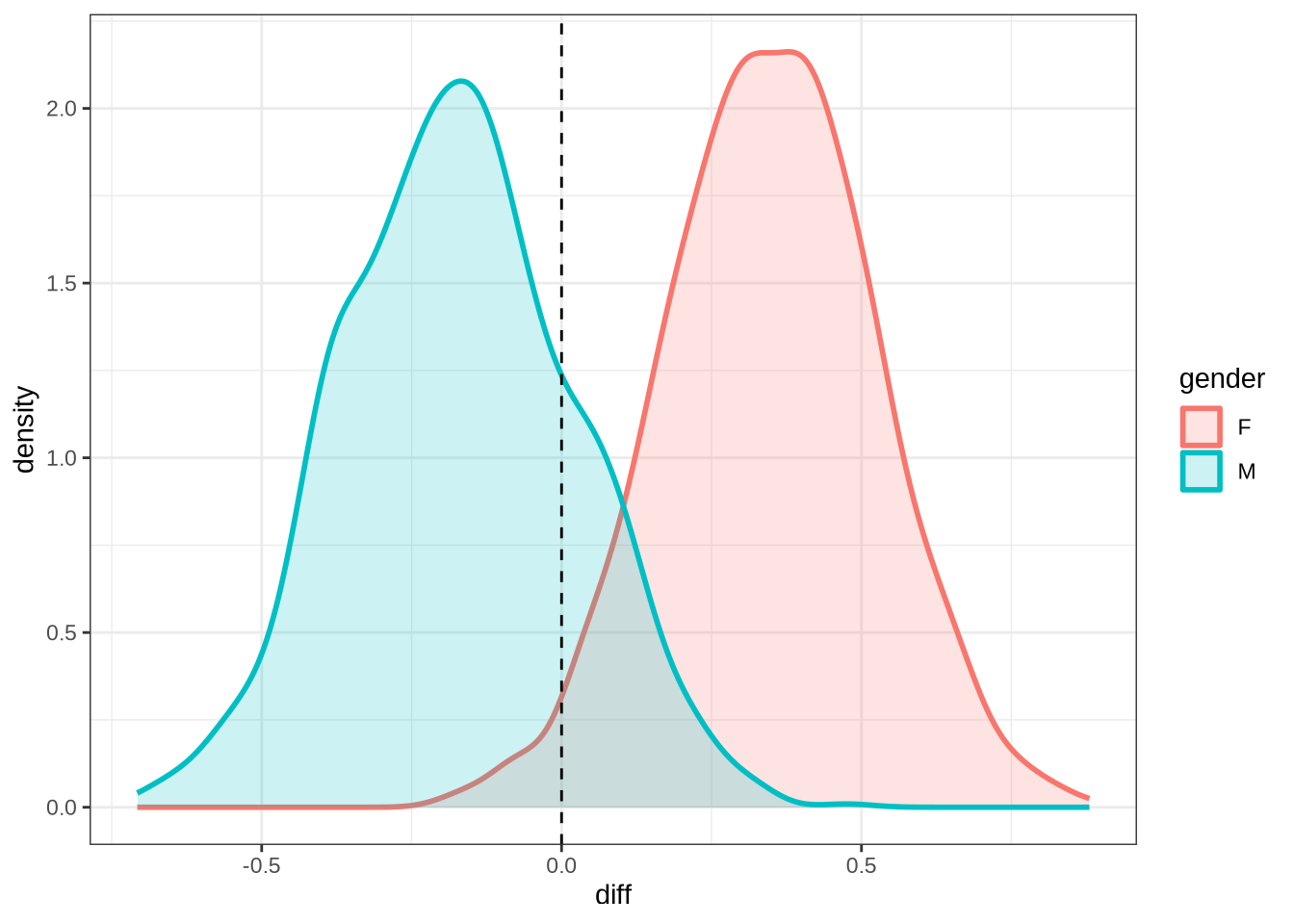
4.1.2.0.8 F2
trap_f2_data <- f2 |>
  filter(
    vowel == "TRAP"
  ) |>
  mutate(
    w_s = interaction(word, stressed),
    p_c = interaction(participant, collect)
  ) %>%
  droplevels()

summary(trap_f2_data)
participant collect age_s gender word
Length:933 Min. :1.000 Min. :-1.8383 F:529 and :391
Class :character 1st Qu.:2.000 1st Qu.:-0.5942 M:404 nana :134
Mode :character Median :3.000 Median : 0.1523 that : 92
Mean :2.875 Mean : 0.0787 back : 57
3rd Qu.:4.000 3rd Qu.: 0.8988 grandma: 26
Max. :4.000 Max. : 2.6405 that's : 23
(Other):210
vowel stressed stopword F2_lob2
TRAP:933 Mode :logical Mode :logical Min. :-2.0312
FALSE:40 FALSE:347 1st Qu.: 0.1073
TRUE :893 TRUE :586 Median : 0.6109
Mean : 0.5612
3rd Qu.: 1.0719
Max. : 3.4007
duration_s age w_s p_c
Min. :-0.79502 Min. :47.0 and.TRUE :375 EC0405-Child.2: 19
1st Qu.:-0.48804 1st Qu.:52.0 nana.TRUE :128 EC0105-Child.2: 18
Median :-0.25780 Median :55.0 that.TRUE : 88 EC2432-Child.3: 18
Mean :-0.11292 Mean :54.7 back.TRUE : 56 EC0118-Child.4: 17
3rd Qu.: 0.05051 3rd Qu.:58.0 grandma.TRUE: 23 EC0520-Child.2: 14
Max. : 2.42830 Max. :65.0 that's.TRUE : 22 EC0607-Child.4: 14
(Other) :241 (Other) :833 trap_f2_fit <- brm(
F2_lob2 ~ gender + stopword +
s(age_s, by=gender, k = 5) +
s(duration_s, k = 5) +
(1 | w_s) +
(1 | p_c),
data = trap_f2_data,
family = student(),
prior = prior_t,
chains = 4,
cores = 4,
iter = 4000,
control = list(adapt_delta = 0.99),
)
write_rds(trap_f2_fit, here('models', 'trap_f2_fit_t.rds'), compress = "gz")trap_f2_fit <- read_rds(here('models', 'trap_f2_fit_t.rds'))summary(trap_f2_fit) Family: student
Links: mu = identity; sigma = identity; nu = identity
Formula: F2_lob2 ~ gender + stopword + s(age_s, by = gender, k = 5) + s(duration_s, k = 5) + (1 | w_s) + (1 | p_c)
Data: trap_f2_data (Number of observations: 933)
Draws: 4 chains, each with iter = 4000; warmup = 2000; thin = 1;
total post-warmup draws = 8000
Smoothing Spline Hyperparameters:
Estimate Est.Error l-95% CI u-95% CI Rhat Bulk_ESS
sds(sage_sgenderF_1) 0.31 0.25 0.01 0.93 1.00 3738
sds(sage_sgenderM_1) 0.33 0.26 0.01 0.96 1.00 4471
sds(sduration_s_1) 0.32 0.26 0.01 0.96 1.00 3805
Tail_ESS
sds(sage_sgenderF_1) 4078
sds(sage_sgenderM_1) 4066
sds(sduration_s_1) 4165
Multilevel Hyperparameters:
~p_c (Number of levels: 185)
Estimate Est.Error l-95% CI u-95% CI Rhat Bulk_ESS Tail_ESS
sd(Intercept) 0.29 0.03 0.23 0.36 1.00 2556 4443
~w_s (Number of levels: 73)
Estimate Est.Error l-95% CI u-95% CI Rhat Bulk_ESS Tail_ESS
sd(Intercept) 0.33 0.08 0.18 0.51 1.00 1845 3455
Regression Coefficients:
Estimate Est.Error l-95% CI u-95% CI Rhat Bulk_ESS Tail_ESS
Intercept 0.60 0.09 0.42 0.78 1.00 4068 5461
genderM -0.20 0.06 -0.32 -0.07 1.00 5517 5741
stopwordTRUE 0.12 0.13 -0.15 0.38 1.00 2911 4651
sage_s:genderF_1 -0.19 0.59 -1.50 0.93 1.00 5107 4322
sage_s:genderM_1 -0.42 0.63 -1.91 0.69 1.00 5147 4523
sduration_s_1 0.11 0.57 -0.84 1.50 1.00 4904 4571
Further Distributional Parameters:
Estimate Est.Error l-95% CI u-95% CI Rhat Bulk_ESS Tail_ESS
sigma 0.47 0.03 0.42 0.53 1.00 3617 5602
nu 3.35 0.49 2.53 4.43 1.00 5504 6609
Draws were sampled using sampling(NUTS). For each parameter, Bulk_ESS
and Tail_ESS are effective sample size measures, and Rhat is the potential
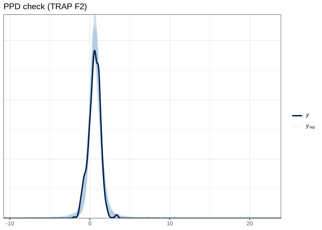
scale reduction factor on split chains (at convergence, Rhat = 1).pp_check(trap_f2_fit, ndraws = 100) +
labs(
title = "PPD check (TRAP F2)"
) 
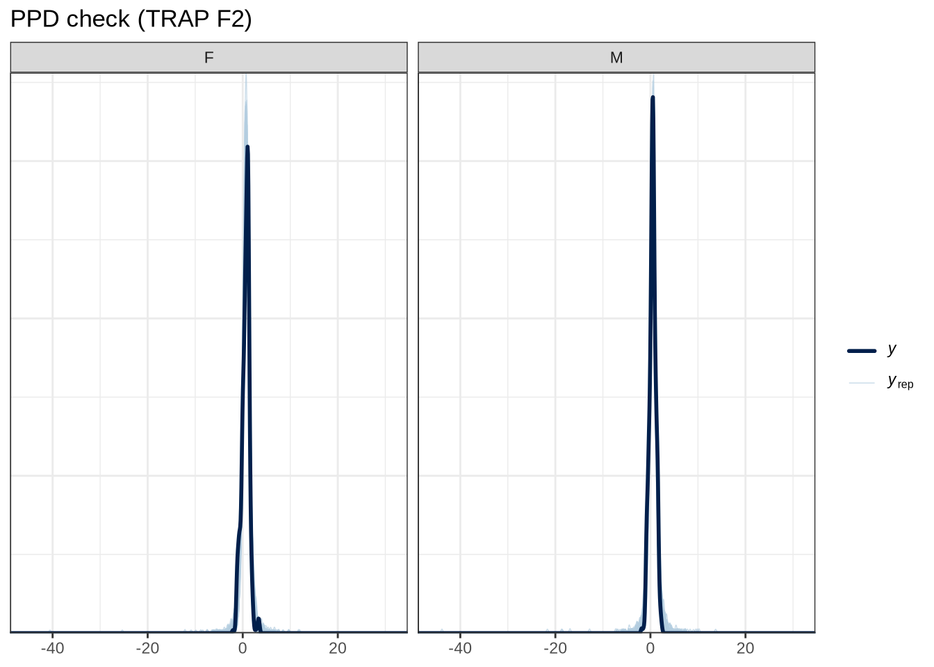
pp_check(trap_f2_fit, type="dens_overlay_grouped", group="gender", ndraws = 100) +
  labs(
    title = "PPD check (TRAP F2)"
  )
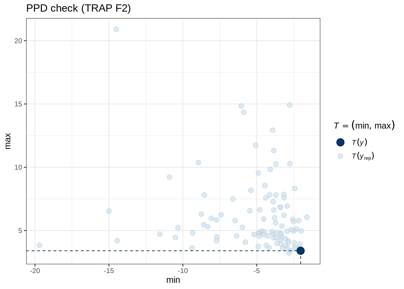
pp_check(trap_f2_fit, type = "stat_2d", stat = c("min", "max"), ndraws = 100) +
  labs(
    title = "PPD check (TRAP F2)"
  )
model_plots(trap_f2_fit) +
  plot_annotation(title = "TRAP F2")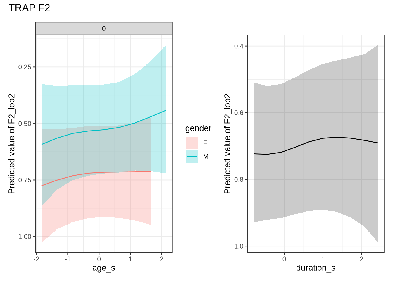
trap_f2_preds <- estimate_relation(
    trap_f2_fit,
    by = list(
      age_s = seq(min_age_s, max_age_s, length = 50),
      gender = c("F", "M"),
      duration_s = 0
    ),
    predict="link",
    ci = c(0.9, 0.7)
  )
trap_f2_10 <- ten_month_preds(trap_f2_fit, sample_points)
trap_f2_10 %>%
ggplot(
aes(
x = diff,
colour = gender,
fill = gender
)
) +
geom_density(linewidth = 1, alpha = 0.2) +
geom_vline(xintercept = 0, linetype = "dashed")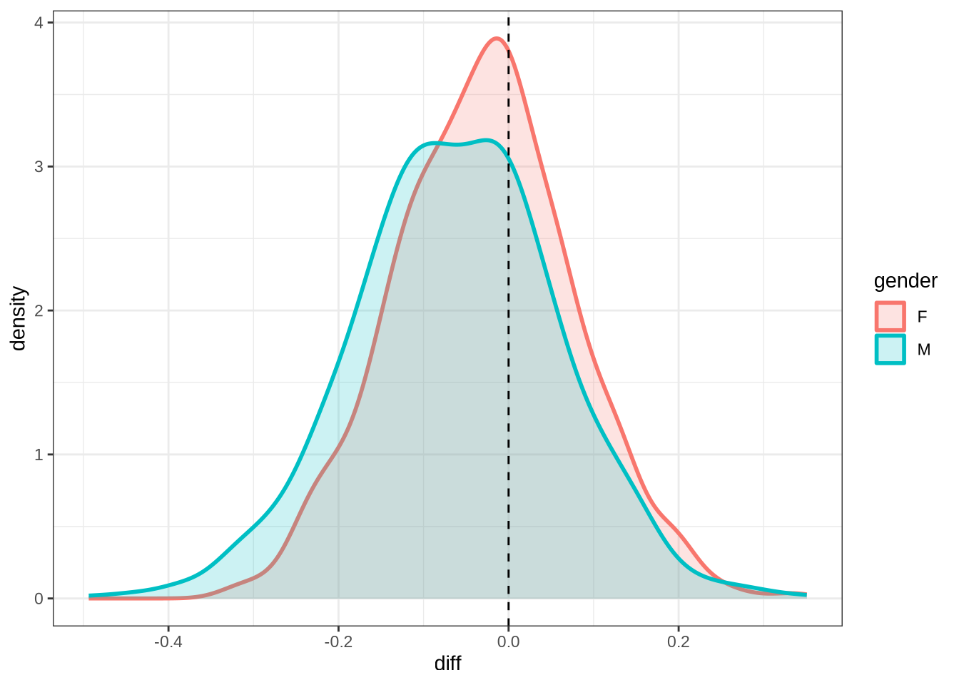
rm(
  trap_f1_fit,
  trap_f2_fit
)
4.1.2.0.9 F1
fleece_f1_data <- f1 |>
  filter(
    vowel == "FLEECE"
  ) |>
  mutate(
    w_s = interaction(word, stressed),
    p_c = interaction(participant, collect)
  ) %>%
  droplevels()


summary(fleece_f1_data)
participant collect age_s gender word
Length:1116 Min. :1.000 Min. :-1.83828 F:595 he :440
Class :character 1st Qu.:2.000 1st Qu.:-0.84298 M:521 the :189
Mode :character Median :3.000 Median :-0.09651 she :174
Mean :2.849 Mean : 0.01162 tui : 65
3rd Qu.:4.000 3rd Qu.: 0.64996 he's : 34
Max. :4.000 Max. : 2.14290 see : 29
(Other):185
vowel stressed stopword F1_lob2
FLEECE:1116 Mode :logical Mode :logical Min. :-3.7569
FALSE:129 FALSE:238 1st Qu.:-1.5829
TRUE :987 TRUE :878 Median :-1.1389
Mean :-1.0330
3rd Qu.:-0.5608
Max. : 3.6886
duration_s age w_s p_c
Min. :-1.0124 Min. :47.00 he.TRUE :427 EC0405-Child.2: 24
1st Qu.:-0.6548 1st Qu.:51.00 the.TRUE :181 EC1522-Child.1: 19
Median :-0.2972 Median :54.00 she.TRUE :171 EC0413-Child.3: 18
Mean :-0.1098 Mean :54.43 tui.FALSE: 65 EC2432-Child.3: 17
3rd Qu.: 0.2392 3rd Qu.:57.00 he's.TRUE: 33 EC0914-Child.4: 17
Max. : 2.3906 Max. :63.00 see.TRUE : 28 EC1106-Child.4: 17
(Other) :211 (Other) :1004 fleece_f1_fit <- brm(
F1_lob2 ~ gender + stopword +
s(age_s, by=gender, k = 5) +
s(duration_s, k = 5) +
(1 | w_s) +
(1 | p_c),
data = fleece_f1_data,
family = student(),
prior = prior_t,
chains = 4,
cores = 4,
iter = 3000,
control = list(adapt_delta = 0.9),
)
write_rds(fleece_f1_fit, here('models', 'fleece_f1_fit_t.rds'), compress = "gz")fleece_f1_fit <- read_rds(here('models', 'fleece_f1_fit_t.rds'))summary(fleece_f1_fit) Family: student
Links: mu = identity; sigma = identity; nu = identity
Formula: F1_lob2 ~ gender + stopword + s(age_s, by = gender, k = 5) + s(duration_s, k = 5) + (1 | w_s) + (1 | p_c)
Data: fleece_f1_data (Number of observations: 1116)
Draws: 4 chains, each with iter = 3000; warmup = 1500; thin = 1;
total post-warmup draws = 6000
Smoothing Spline Hyperparameters:
Estimate Est.Error l-95% CI u-95% CI Rhat Bulk_ESS
sds(sage_sgenderF_1) 0.32 0.27 0.01 0.99 1.00 2552
sds(sage_sgenderM_1) 0.28 0.23 0.01 0.84 1.00 3025
sds(sduration_s_1) 0.47 0.30 0.03 1.16 1.00 1965
Tail_ESS
sds(sage_sgenderF_1) 2735
sds(sage_sgenderM_1) 2840
sds(sduration_s_1) 1809
Multilevel Hyperparameters:
~p_c (Number of levels: 187)
Estimate Est.Error l-95% CI u-95% CI Rhat Bulk_ESS Tail_ESS
sd(Intercept) 0.28 0.03 0.21 0.34 1.00 1912 3356
~w_s (Number of levels: 64)
Estimate Est.Error l-95% CI u-95% CI Rhat Bulk_ESS Tail_ESS
sd(Intercept) 0.38 0.06 0.27 0.51 1.00 2157 3388
Regression Coefficients:
Estimate Est.Error l-95% CI u-95% CI Rhat Bulk_ESS Tail_ESS
Intercept -1.06 0.09 -1.24 -0.88 1.00 3596 4341
genderM -0.02 0.06 -0.14 0.10 1.00 2940 3482
stopwordTRUE 0.02 0.16 -0.29 0.33 1.00 1808 2635
sage_s:genderF_1 -0.62 0.55 -1.84 0.47 1.00 3080 3001
sage_s:genderM_1 -0.04 0.52 -1.08 1.04 1.00 3750 4180
sduration_s_1 0.02 0.57 -1.09 1.25 1.00 3794 3347
Further Distributional Parameters:
Estimate Est.Error l-95% CI u-95% CI Rhat Bulk_ESS Tail_ESS
sigma 0.54 0.02 0.49 0.58 1.00 3090 4178
nu 3.82 0.51 2.94 4.93 1.00 4026 4219
Draws were sampled using sampling(NUTS). For each parameter, Bulk_ESS
and Tail_ESS are effective sample size measures, and Rhat is the potential
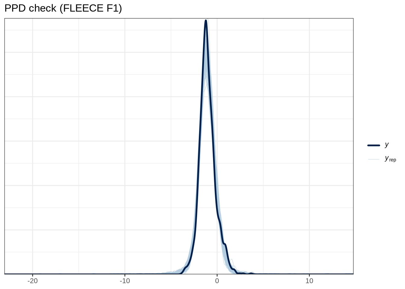
scale reduction factor on split chains (at convergence, Rhat = 1).pp_check(fleece_f1_fit, ndraws = 100) +
labs(
title = "PPD check (FLEECE F1)"
) 
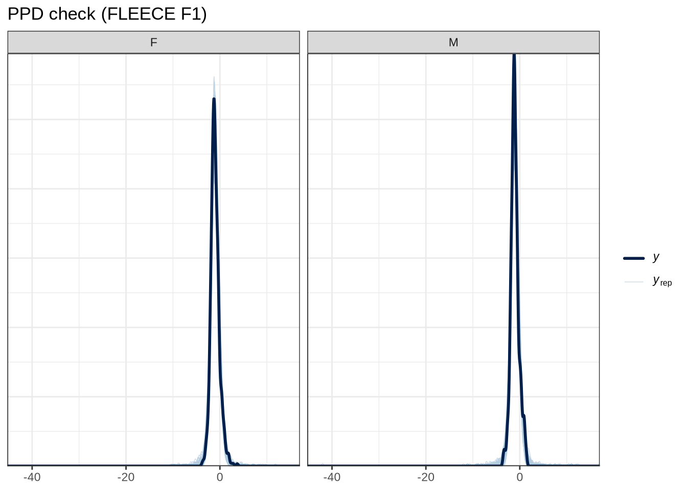
pp_check(fleece_f1_fit, type="dens_overlay_grouped", group="gender", ndraws = 100) +
  labs(
    title = "PPD check (FLEECE F1)"
  )
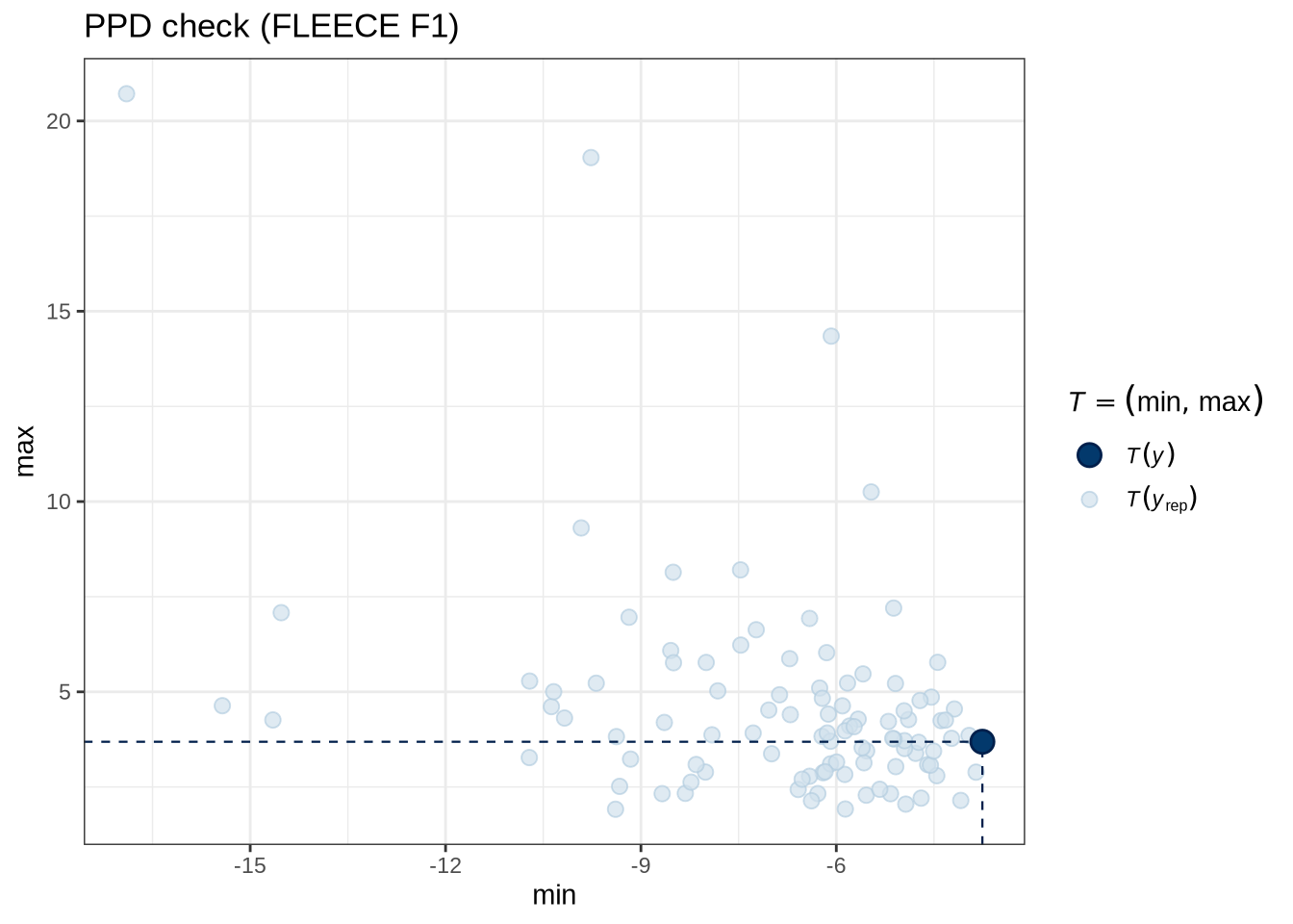
pp_check(fleece_f1_fit, type = "stat_2d", stat = c("min", "max"), ndraws = 100) +
  labs(
    title = "PPD check (FLEECE F1)"
  )
model_plots(fleece_f1_fit) +
  plot_annotation(title = "FLEECE F1")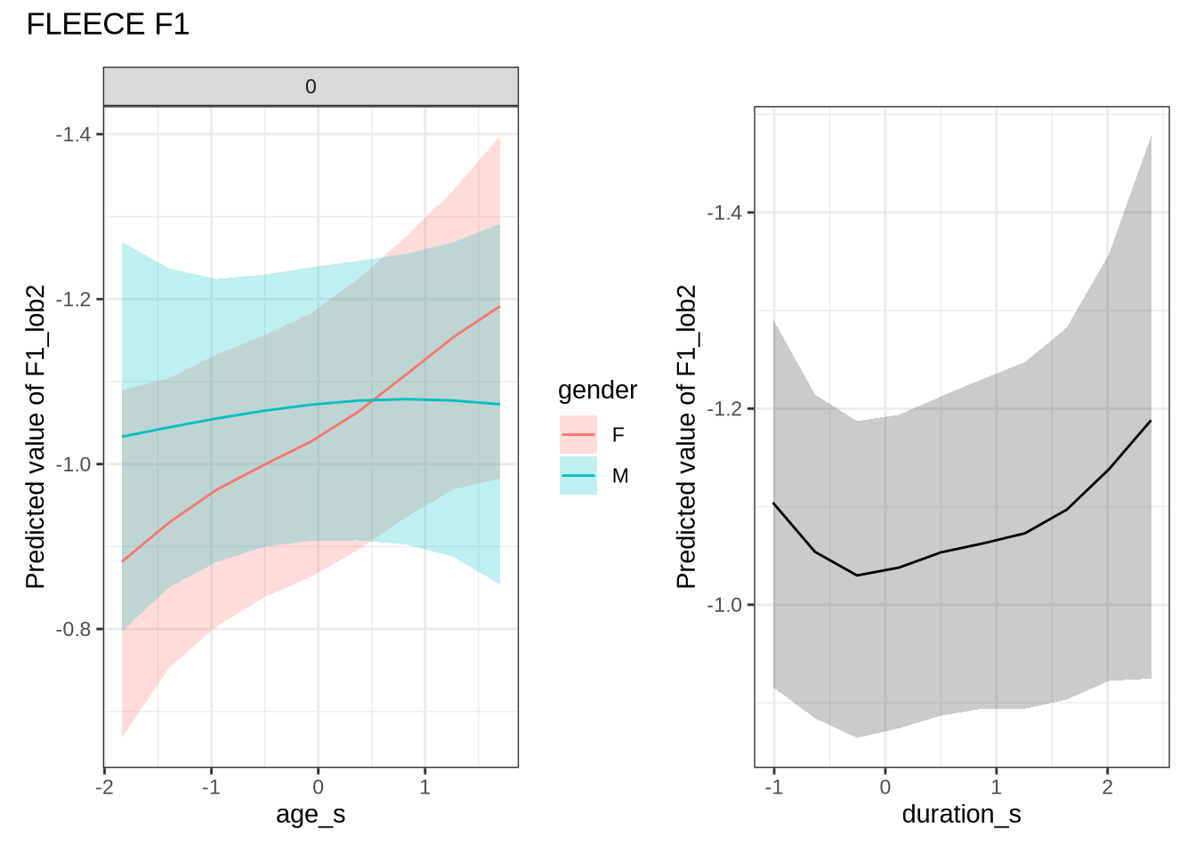
fleece_f1_preds <- estimate_relation(
    fleece_f1_fit,
    by = list(
      age_s = seq(min_age_s, max_age_s, length = 50),
      gender = c("F", "M"),
      duration_s = 0
    ),
    predict="link",
    ci = c(0.9, 0.7)
)diff_check(fleece_f1_fit, fleece_f1_data) %>%
diff_plot()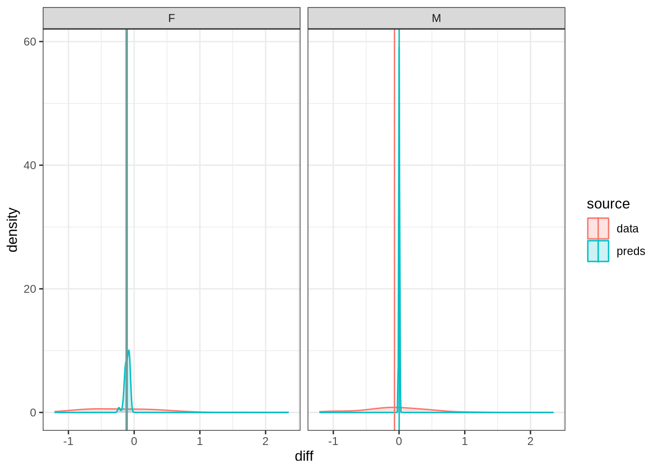
We claim F1 movement for female preschoolers in the paper and this matches the mean difference for female preschoolers when the data is viewed longitudinally.
fleece_f1_10 <- ten_month_preds(fleece_f1_fit, sample_points)
fleece_f1_10 %>%
  ggplot(
    aes(
      x = diff,
      colour = gender,
      fill = gender
    )
  ) +
  geom_density(linewidth = 1, alpha = 0.2) +
  geom_vline(xintercept = 0, linetype = "dashed")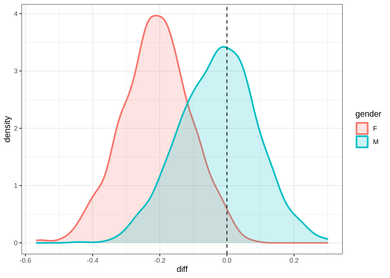
4.1.2.0.10 F2
fleece_f2_data <- f2 |>
  filter(
    vowel == "FLEECE"
  ) |>
  mutate(
    w_s = interaction(word, stressed),
    p_c = interaction(participant, collect)
  ) %>%
  droplevels()

summary(fleece_f2_data)
participant collect age_s gender word
Length:1122 Min. :1.000 Min. :-1.83828 F:604 he :434
Class :character 1st Qu.:2.000 1st Qu.:-0.84298 M:518 the :195
Mode :character Median :3.000 Median :-0.09651 she :174
Mean :2.835 Mean : 0.01748 tui : 63
3rd Qu.:4.000 3rd Qu.: 0.83658 he's : 34
Max. :4.000 Max. : 2.64055 see : 29
(Other):193
vowel stressed stopword F2_lob2
FLEECE:1122 Mode :logical Mode :logical Min. :-1.8707
FALSE:126 FALSE:237 1st Qu.: 0.7638
TRUE :996 TRUE :885 Median : 1.6287
Mean : 1.4433
3rd Qu.: 2.1565
Max. : 5.2232
duration_s age w_s p_c
Min. :-1.0124 Min. :47.00 he.TRUE :421 EC0405-Child.2: 24
1st Qu.:-0.6520 1st Qu.:51.00 the.TRUE :187 EC1522-Child.1: 20
Median :-0.2913 Median :54.00 she.TRUE :171 EC2432-Child.3: 19
Mean :-0.1098 Mean :54.46 tui.FALSE: 63 EC0914-Child.4: 18
3rd Qu.: 0.1917 3rd Qu.:57.75 he's.TRUE: 33 EC0413-Child.3: 17
Max. : 2.3849 Max. :65.00 see.TRUE : 28 EC1106-Child.4: 17
(Other) :219 (Other) :1007 fleece_f2_fit <- brm(
F2_lob2 ~ gender + stopword +
s(age_s, by=gender, k = 5) +
s(duration_s, k = 5) +
(1 | w_s) +
(1 | p_c),
data = fleece_f2_data,
family = student(),
prior = prior_t,
chains = 4,
cores = 4,
iter = 4000,
control = list(adapt_delta = 0.9),
)
write_rds(
fleece_f2_fit,
here('models', 'fleece_f2_fit_t.rds'),
compress = "gz"
)fleece_f2_fit <- read_rds(here('models', 'fleece_f2_fit_t.rds'))summary(fleece_f2_fit) Family: student
Links: mu = identity; sigma = identity; nu = identity
Formula: F2_lob2 ~ gender + stopword + s(age_s, by = gender, k = 5) + s(duration_s, k = 5) + (1 | w_s) + (1 | p_c)
Data: fleece_f2_data (Number of observations: 1122)
Draws: 4 chains, each with iter = 4000; warmup = 2000; thin = 1;
total post-warmup draws = 8000
Smoothing Spline Hyperparameters:
Estimate Est.Error l-95% CI u-95% CI Rhat Bulk_ESS
sds(sage_sgenderF_1) 0.41 0.27 0.02 1.04 1.00 4526
sds(sage_sgenderM_1) 0.33 0.26 0.01 0.96 1.00 4915
sds(sduration_s_1) 0.44 0.25 0.05 1.01 1.00 4870
Tail_ESS
sds(sage_sgenderF_1) 4159
sds(sage_sgenderM_1) 4167
sds(sduration_s_1) 3511
Multilevel Hyperparameters:
~p_c (Number of levels: 188)
Estimate Est.Error l-95% CI u-95% CI Rhat Bulk_ESS Tail_ESS
sd(Intercept) 0.29 0.03 0.22 0.35 1.00 2784 4569
~w_s (Number of levels: 63)
Estimate Est.Error l-95% CI u-95% CI Rhat Bulk_ESS Tail_ESS
sd(Intercept) 0.57 0.08 0.44 0.74 1.00 4050 5997
Regression Coefficients:
Estimate Est.Error l-95% CI u-95% CI Rhat Bulk_ESS Tail_ESS
Intercept 1.55 0.12 1.33 1.77 1.00 5561 5999
genderM 0.00 0.06 -0.12 0.13 1.00 6869 6404
stopwordTRUE -0.21 0.21 -0.62 0.18 1.00 3063 4468
sage_s:genderF_1 -0.46 0.66 -1.85 0.93 1.00 7808 5177
sage_s:genderM_1 -0.11 0.63 -1.39 1.17 1.00 7533 5350
sduration_s_1 0.25 0.58 -0.99 1.35 1.00 9502 6025
Further Distributional Parameters:
Estimate Est.Error l-95% CI u-95% CI Rhat Bulk_ESS Tail_ESS
sigma 0.51 0.03 0.45 0.56 1.00 4611 5943
nu 2.70 0.32 2.15 3.38 1.00 6242 6084
Draws were sampled using sampling(NUTS). For each parameter, Bulk_ESS
and Tail_ESS are effective sample size measures, and Rhat is the potential
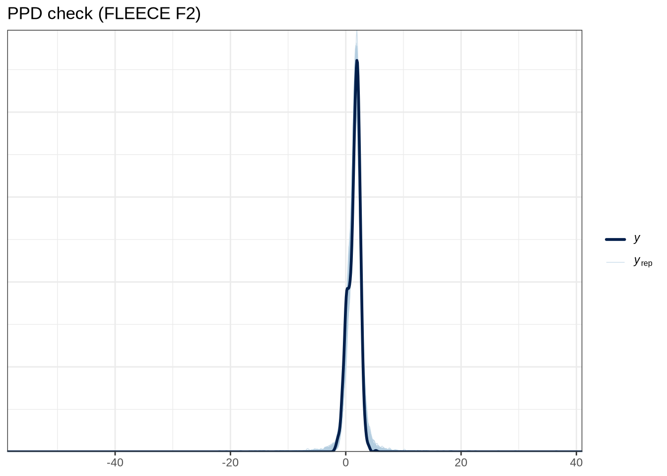
scale reduction factor on split chains (at convergence, Rhat = 1).pp_check(fleece_f2_fit, ndraws = 100) +
labs(
title = "PPD check (FLEECE F2)"
) 
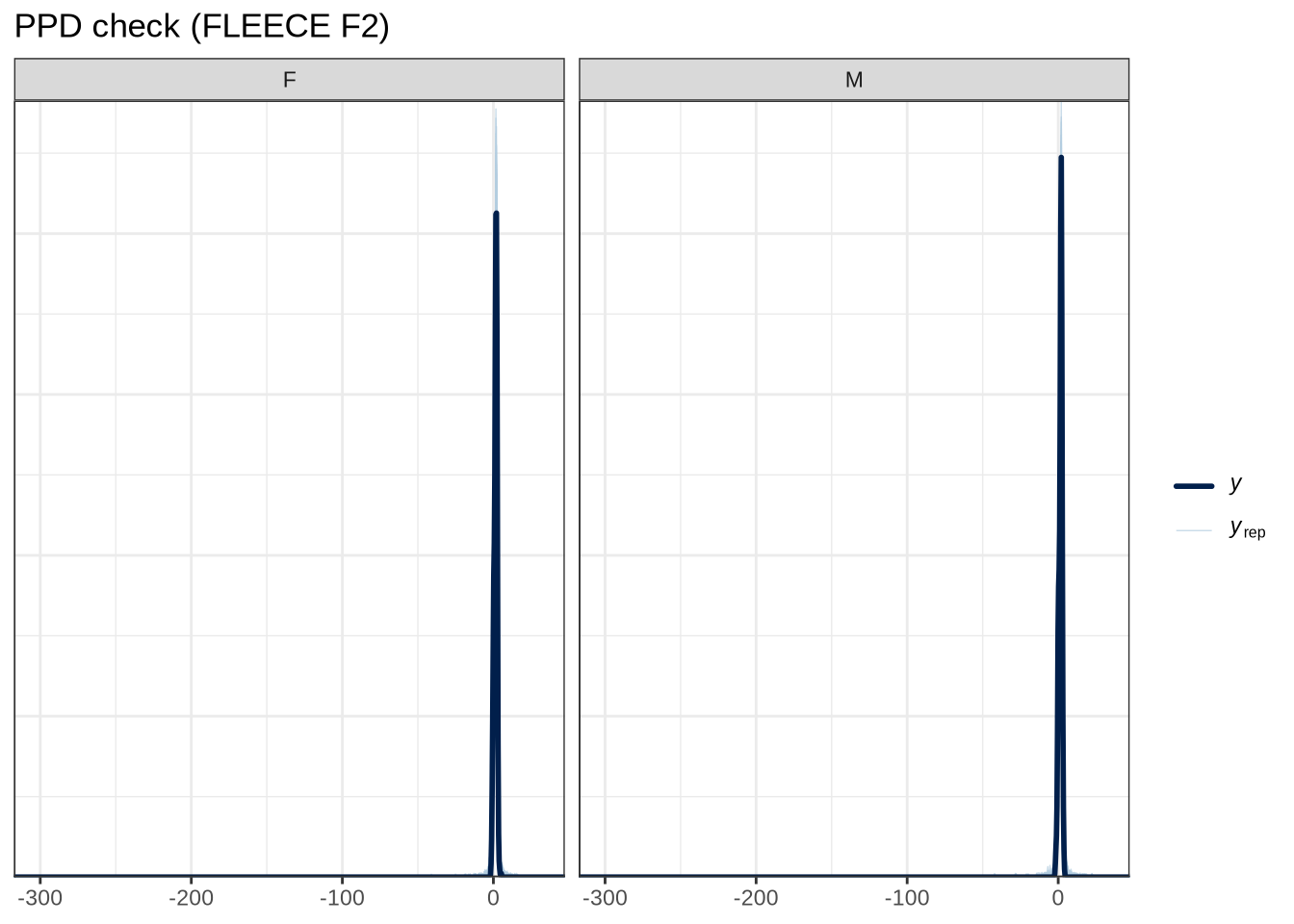
pp_check(fleece_f2_fit, type="dens_overlay_grouped", group="gender", ndraws = 100) +
  labs(
    title = "PPD check (FLEECE F2)"
  )
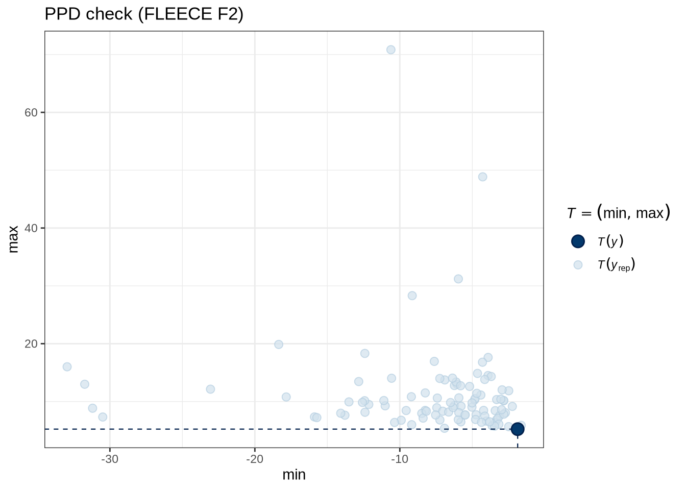
pp_check(fleece_f2_fit, type = "stat_2d", stat = c("min", "max"), ndraws = 100) +
  labs(
    title = "PPD check (FLEECE F2)"
  )
model_plots(fleece_f2_fit) +
  plot_annotation(title = "FLEECE F2")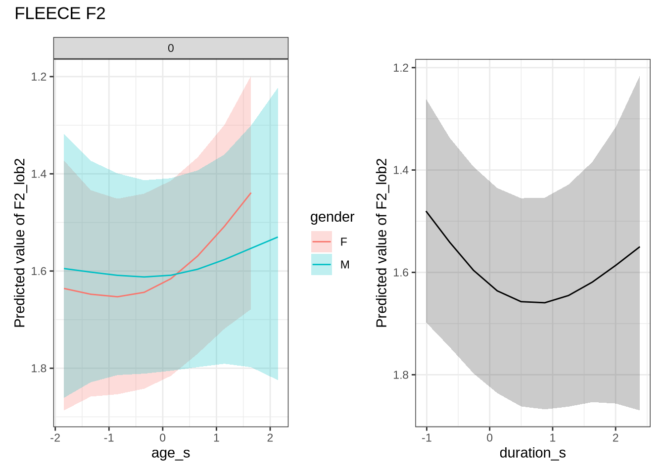
fleece_f2_preds <- estimate_relation(
    fleece_f2_fit,
    by = list(
      age_s = seq(min_age_s, max_age_s, length = 50),
      gender = c("F", "M"),
      duration_s = 0
    ),
    predict="link",
    ci = c(0.9, 0.7)
  )
fleece_f2_10 <- ten_month_preds(fleece_f2_fit, sample_points)
fleece_f2_10 %>%
ggplot(
aes(
x = diff,
colour = gender,
fill = gender
)
) +
geom_density(linewidth = 1, alpha = 0.2) +
geom_vline(xintercept = 0, linetype = "dashed")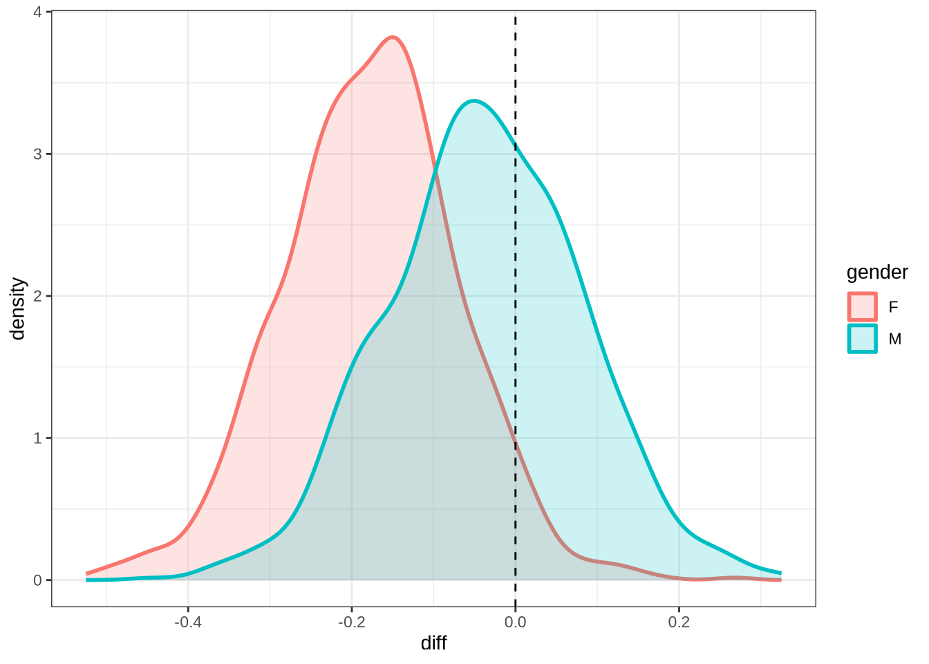
rm(fleece_f1_fit, fleece_f2_fit)4.2 Summary Plots
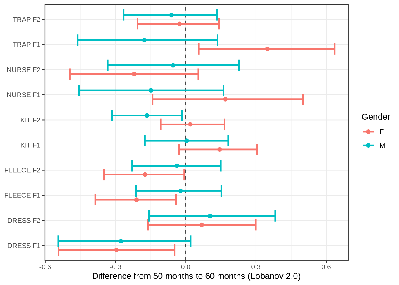
Let’s plot differences from 50 to 60 months for all models and then for the models which we have identified for the paper.
age_change_preds <- list_rbind(
  list(
    "DRESS F1" = dress_f1_10,
    "DRESS F2" = dress_f2_10,
    "KIT F1" = kit_f1_10,
    "KIT F2" = kit_f2_10,
    "NURSE F1" = nurse_f1_10,
    "NURSE F2" = nurse_f2_10,
    "TRAP F1" = trap_f1_10,
    "TRAP F2" = trap_f2_10,
    "FLEECE F1" = fleece_f1_10,
    "FLEECE F2" = fleece_f2_10
  ),
  names_to = "variable"
)

age_change_preds %>%
  group_by(variable, gender) %>%
  summarise(
    median = median(diff),
    fifth = quantile(diff, probs = 0.05),
    ninetyfifth = quantile(diff, probs = 0.95)
  ) %>%
  ggplot(
    aes(
      y = variable,
      x = median,
      xmin = fifth,
      xmax = ninetyfifth,
      colour = gender
    )
  ) +
  geom_vline(xintercept = 0, linetype = "dashed") +
  geom_errorbar(position = position_dodge(width=0.7), linewidth=1) +
  geom_point(position = position_dodge(width=0.7), size=2) +
  labs(
    x = "Difference from 50 months to 60 months (Lobanov 2.0)",
    y = NULL,
    colour = "Gender"
  )
Now the specific variables.
subset_change <- age_change_preds %>%
  filter(
    variable %in% c("DRESS F1", "FLEECE F1", "KIT F1", "KIT F2")
  ) %>%
  group_by(variable, gender) %>%
  summarise(
    median = median(diff),
    fifth = quantile(diff, probs = 0.05),
    ninetyfifth = quantile(diff, probs = 0.95)
  ) %>%
  ggplot(
    aes(
      y = variable,
      x = median,
      xmin = fifth,
      xmax = ninetyfifth,
      colour = gender
    )
  ) +
  geom_vline(xintercept = 0, linetype = "dashed") +
  geom_errorbar(position = position_dodge(width=0.7), linewidth=1) +
  geom_point(position = position_dodge(width=0.7), size=2) +
  labs(
    x = "Difference from 50 months to 60 months (Lobanov 2.0)",
    y = NULL,
    colour = "Gender"
  )

ggsave(
  filename = here('plots', 'figure6_tenmonth.tiff'),
  plot = subset_change,
  width = 7,
  height = 5,
  dpi = 300
)

subset_change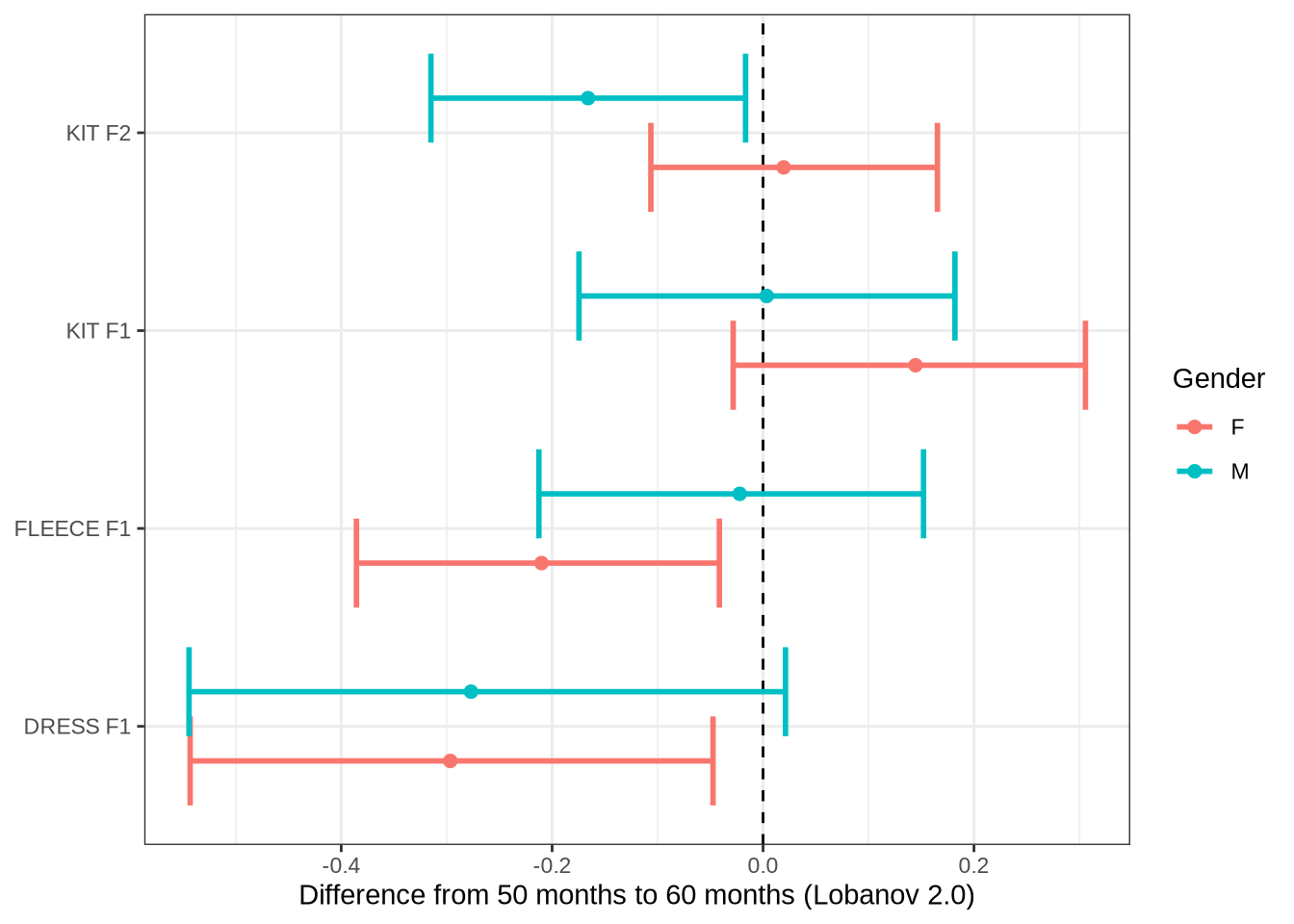
5 QuakeBox models
5.1 Fit
Here we fit GAMM models with similar structures to the QuakeBox (QB). We borrow code from another project (Hurring et al. 2025). We modify the anonymisation script from that project in order to create a stopword variable.
This is a very long section of code, so we have ‘folded’ it by default. First we load up the data and output some token counts which we will add to the paper.
To view code click here
# Check age factor is in the right order.
QB1$age |> factor() |> levels()
[1] "18-25" "26-35" "36-45" "46-55" "56-65" "66-75" "76-85" "85+" To view code click here
# [1] "18-25" "26-35" "36-45" "46-55" "56-65" "66-75" "76-85" "85+"
# yes

# Various variable changes in order to fit a GAMM. We scale variables in
# order to improve model fit and ease of interpretation.
QB1 <- QB1 |>
  mutate(
    age_category_numeric = as.integer(factor(age)),
    speaker = as.factor(speaker),
    gender = as.factor(gender),
    word = as.factor(word),
    stopword = as.factor(stopword),
    stressed = as.factor(!unstressed),
    log_freq = log(celex_frequency + 1),
    log_freq_s = scale(log_freq)[,1],
    age_cat_s = scale(age_category_numeric)[,1],
    w_s = interaction(word, stressed)
  ) %>%
  group_by(vowel) %>%
  mutate(
    duration_s = scale(vowel_end - vowel_start)[,1]
  ) %>%
  filter(
    duration_s < 2.5
  ) %>%
  ungroup()

QB1_caregivercount <- QB1 |>
  filter(
    vowel %in% c(
      "DRESS",
      "FLEECE",
      "TRAP",
      "KIT",
      "NURSE"
    ),
    gender == "f",
    age_category_numeric %in% c(1, 2)
  ) |>
  mutate(
    n = n_distinct(speaker)
  )
# 24627 tokens from notional caregiver generation.
cat('Tokens from caregiver generation: ', nrow(QB1_caregivercount), '\n')
Tokens from caregiver generation: 24119 To view code click here
QB1_oldestgeneration <- QB1 |>
  filter(
    vowel %in% c(
      "DRESS",
      "FLEECE",
      "TRAP",
      "KIT",
      "NURSE"
    ),
    gender == "f",
    age_category_numeric %in% c(7, 8)
  ) |>
  mutate(
    n = n_distinct(speaker)
  )
# 4992 tokens from oldest generation.
cat('Tokens from oldest generation: ', nrow(QB1_oldestgeneration), '\n')
Tokens from oldest generation: 4914 To view code click here
# 45 speakers in notional caregiver generation.
cat('Caregivers: ', QB1_caregivercount$n[[1]], '\n')
Caregivers: 45 To view code click here
# 18 speakers in oldest generation
cat('Oldest: ', QB1_oldestgeneration$n[[1]])
Oldest: 10We output some further information for tables in the paper:
QB1 %>%
  group_by(speaker) %>%
  summarise(gender = first(gender)) %>%
  count(gender)
# A tibble: 2 × 2
gender n
<fct> <int>
1 f 235
2 m 110What are the counts for each vowel category?
# front vowel counts
qb_counts <- QB1 %>%
  count(vowel)

qb_counts
# A tibble: 10 × 2
vowel n
<fct> <int>
1 TRAP 62340
2 START 13166
3 THOUGHT 15269
4 NURSE 12389
5 DRESS 29495
6 FLEECE 52437
7 KIT 101280
8 LOT 47425
9 GOOSE 25406
10 STRUT 42779How many speakers are there in each age and gender category?
QB1 %>%
  group_by(age, gender) %>%
  summarise(
    n_speakers = n_distinct(speaker)
  )
# A tibble: 16 × 3
# Groups: age [8]
age gender n_speakers
<chr> <fct> <int>
1 18-25 f 30
2 18-25 m 21
3 26-35 f 15
4 26-35 m 7
5 36-45 f 43
6 36-45 m 15
7 46-55 f 56
8 46-55 m 23
9 56-65 f 50
10 56-65 m 18
11 66-75 f 31
12 66-75 m 18
13 76-85 f 7
14 76-85 m 6
15 85+ f 3
16 85+ m 2The total number of tokens is 401986. The total number of short front vowel tokens is 257941
Now we fit the models specified here uses nearly 40GB of RAM. Researchers with less access to computation may need to fit the models one-at-a-time rather than keeping all in memory at once. The very large size of these models is due to the complexity of the random effects structure.
relevant_to_fix <- list.files(here('models'), pattern = "QB1", full.names=T)

for (fn in relevant_to_fix) {
  #mod <- read_rds(fn)
  #qs_save(mod, )
  qs2::rds_to_qs(fn, str_replace_all(fn, "rds", "qs2"))
}
To view code click here
QB1_models <- QB1 %>%
  select(
    -F1_50, -F2_50
  ) %>%
  pivot_longer(
    cols = F1_lob2:F2_lob2,
    names_to = "formant_type",
    values_to = "formant_value"
  ) %>%
  group_by(vowel, formant_type) %>%
  nest() %>%
  mutate(
    data = map(data, droplevels),
    model = map2(
      data,
      str_c(vowel, formant_type),
      ~ {
        if (file.exists(
          here('models', paste0('QB1_', .y, '_t.qs2'))
        )) {
          mod <- qs_read(here('models', paste0('QB1_', .y, '_t.qs2')))
        } else {

          mod <- brm(
            formant_value ~ gender + stopword +
              s(age_cat_s, by=gender, k = 5) +
              s(duration_s, k = 5) +
              (1 | w_s) +
              (1 | speaker),
            data = .x,
            family = student(),
            prior = prior_t,
            chains = 4,
            cores = 4,
            iter = 2000,
            control = list(adapt_delta = 0.99)
          )

        qs_save(mod, here('models', paste0('QB1_', .y, '_t.qs2')), nthreads=8L)
      }

      mod
      }
    )
  )
5.2 Diagnostics
We’ll have a quick look at some posterior predictive checks.
ppd_plots <- list()
for (i in 1:nrow(QB1_models)) {
  (
    ppd_plot <- pp_check(
      QB1_models$model[[i]],
      type="dens_overlay_grouped",
      group="gender",
      ndraws = 100
    ) +
    labs(
      title = "PPD check (DRESS F1)"
    )
  )
  ppd_plots <- append(ppd_plots, ppd_plot)
}

write_rds(ppd_plots, here('data', 'ppd_plots.rds'))
There’s nothing obviously bad here. There is an issue with t-distributions for responses is that (by design) they allow large outliers. If you sample from t-distributions multiples times, you will get some crazy values. This explains the large x-axis range.
5.3 Generate predictions and plot
First, as a sanity check, we’ll look at QB1 change over age categories.
test <- estimate_relation(
  QB1_models$model[[11]],
  by = c("age_cat_s = seq(-1.79693581, 2.55572475, 0.6218086)", "gender", "duration_s = 0"),
  predict="link",
  ci = 0.9
)

test
Model-based Predictions
age_cat_s | gender | duration_s | Predicted | SE | CI
-------------------------------------------------------------------
-1.80 | f | 0 | -0.82 | 0.03 | [-0.87, -0.77]
-1.18 | f | 0 | -0.79 | 0.02 | [-0.83, -0.76]
-0.55 | f | 0 | -0.79 | 0.02 | [-0.82, -0.75]
0.07 | f | 0 | -0.82 | 0.02 | [-0.85, -0.79]
0.69 | f | 0 | -0.86 | 0.02 | [-0.89, -0.83]
1.31 | f | 0 | -0.91 | 0.02 | [-0.95, -0.87]
1.93 | f | 0 | -0.97 | 0.04 | [-1.03, -0.91]
-1.80 | m | 0 | -1.07 | 0.04 | [-1.13, -1.01]
-1.18 | m | 0 | -1.00 | 0.03 | [-1.06, -0.95]
-0.55 | m | 0 | -0.98 | 0.04 | [-1.04, -0.92]
0.07 | m | 0 | -1.01 | 0.03 | [-1.05, -0.96]
0.69 | m | 0 | -1.05 | 0.03 | [-1.10, -1.01]
1.31 | m | 0 | -1.07 | 0.03 | [-1.12, -1.02]
1.93 | m | 0 | -1.06 | 0.04 | [-1.13, -0.99]
Variable predicted: formant_value
Predictors modulated: age_cat_s = seq(-1.79693581, 2.55572475, 0.6218086), gender, duration_s = 0
Predictors controlled: stopword (FALSE)
Predictions are on the link-scale.plot(test) +
labs(
title = QB1_models$vowel[[1]],
subtitle = QB1_models$formant_type[[1]]
)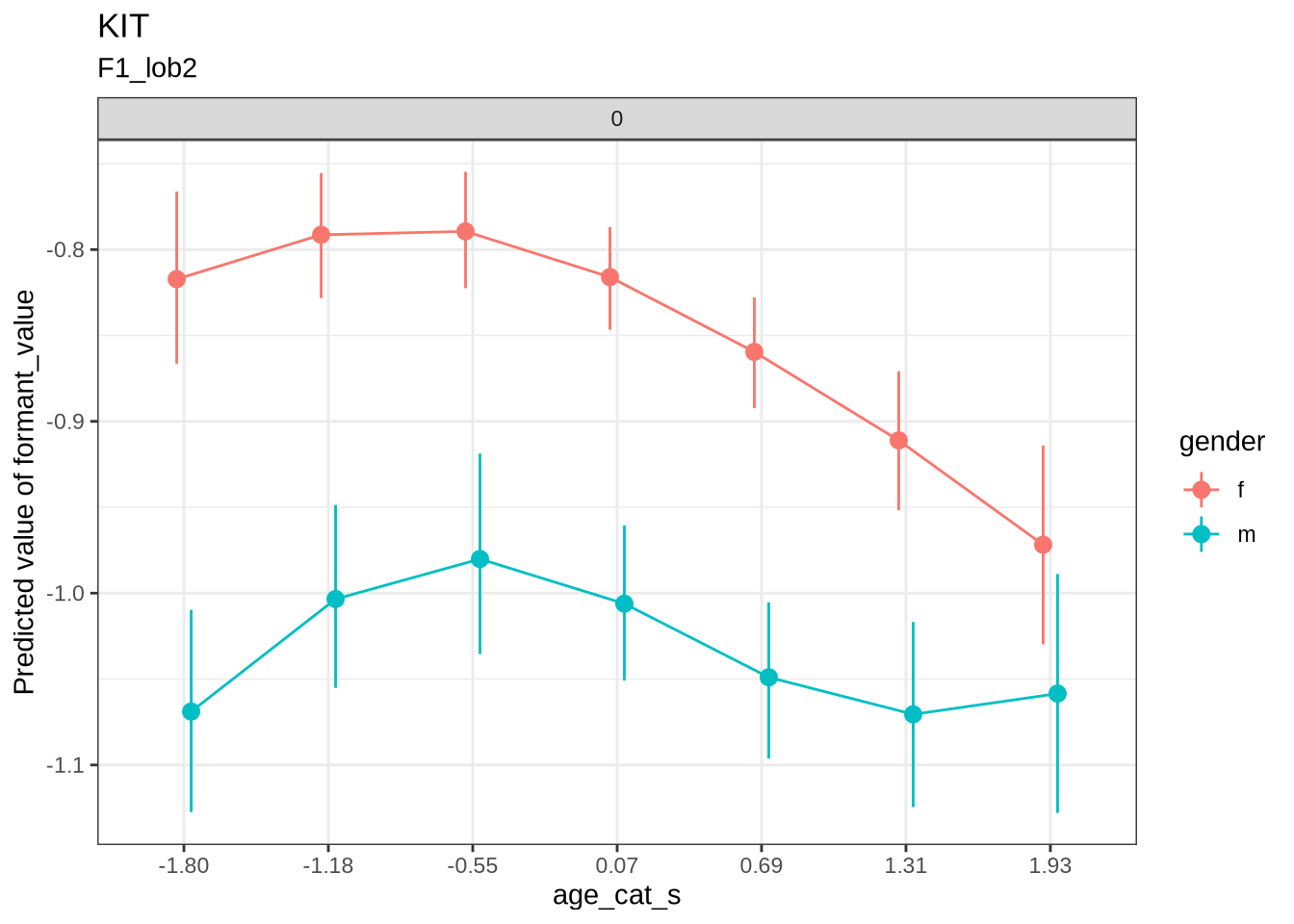
We do the same for each individual model. First we extract the predictions.
QB1_preds <- QB1_models %>%
  mutate(
    preds = map(
      model,
      ~ estimate_relation(
        .x,
        by = c("age_cat_s = seq(-1.79693581, 2.55572475, 0.6218086/4)", "gender", "duration_s = 0"),
        predict="link",
        ci = c(0.6, 0.8, 0.9)
      )
    )
  ) %>%
  select(
    preds
  ) %>%
  unnest(preds)

# Unstandardise
QB1_preds <- QB1_preds %>%
  mutate(
    age_cat = mean(QB1$age_category_numeric) + age_cat_s * sd(QB1$age_category_numeric)
  )

QB1_preds <- QB1_preds %>%
  pivot_wider(
    names_from = formant_type,
    values_from = c(Predicted, SE, contains("CI"))
  ) %>%
  arrange(desc(age_cat))

QB1_preds %>%
  ggplot(
    aes(
      x = Predicted_F2_lob2,
      y = Predicted_F1_lob2,
      colour = vowel,
      group = vowel,
      label = vowel
    )
  ) +
  geom_path(linewidth=1, arrow = arrow(length = unit(2, "mm"))) +
  geom_label(size = 2, data = QB1_preds %>% filter(age_cat == max(age_cat))) +
  scale_y_reverse() +
  scale_x_reverse() +
  facet_grid(cols = vars(gender)) +
  theme(legend.position = "none")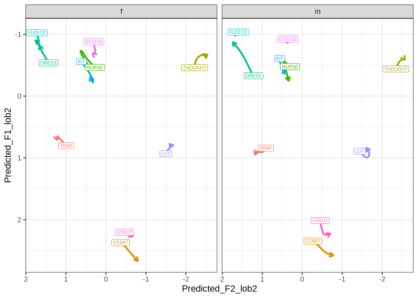
(figs-qb1-change-time?) doesn’t show anything too surprising given previous research.
Create columns to identify reference predictions.
QB1_preds <- QB1_preds %>%
  mutate(
    generation = case_when(
      between(age_cat, 6.9, 8) & gender == "f" ~ "Oldest",
      between(age_cat, 0.9, 2.1) & gender == "f" ~ "Caregiver",
      .default = "Other"
    )
  )
Now we plot just the extended short front vowel shift.
ci_boxes <- QB1_preds %>%
  group_by(vowel) %>%
  filter(
    age_cat == max(age_cat)
  ) %>%
  mutate(
    gender = if_else(gender == "f", "Female", "Male"),
    gender = factor(gender, levels = c("Female", "Male"))
  ) %>%
  group_by(vowel, gender) %>%
  nest() %>%
  mutate(
    ci_90 = map(
      data,
      ~ {
        points <- .x %>%
          select(
            CI_high_0.9_F2_lob2, CI_low_0.9_F2_lob2,
            CI_high_0.9_F1_lob2, CI_low_0.9_F1_lob2
          ) %>%
          pivot_longer(
            cols = everything(),
            names_to = "type",
            values_to = "value"
          ) %>%
          mutate(
            formant = str_extract(type, "F[1-2]")
          ) %>%
          select(formant, value)
        out <- crossing(
          "F1" = points %>%
            filter(formant == "F1") %>%
            pull(value),
          "F2" = points %>%
            filter(formant == "F2") %>%
            pull(value)
        )
        out %>%
          # order correctly for polygon.
          slice(c(1, 2, 4, 3, 1))
      }
    )
  ) %>%
  select(-data) %>%
  unnest(ci_90) %>%
  filter(
    vowel %in% short_front
  )

QB1_plot <- QB1_preds %>%
  filter(
    vowel %in% short_front
  ) %>%
  mutate(
    label = if_else(age_cat == max(age_cat), vowel, ""),
    gender = if_else(gender == "f", "Female", "Male"),
    gender = factor(gender, levels = c("Female", "Male"))
  ) %>%
  ggplot(
    aes(
      x = Predicted_F2_lob2,
      y = Predicted_F1_lob2,
      colour = vowel,
      group = vowel,
      label = label
    )
  ) +
  geom_point(data = ~.x %>% filter(age_cat == max(age_cat))) +
  geom_textpath(
    aes(
      x = F2,
      y = F1,
      colour = vowel
    ),
    label = "90% CI",
    linetype = "dashed",
    vjust = 1,
    size = 2.5,
    inherit.aes = FALSE,
    data = ci_boxes
  ) +
  geom_polygon(
    aes(
      x = F2,
      y = F1,
      fill = vowel
    ),
    linewidth = 0,
    alpha = 0.4,
    inherit.aes = FALSE,
    data = ci_boxes
  ) +
  geom_path(linewidth=1, arrow = arrow(length = unit(2, "mm"), type = "closed")) +
  geom_label_repel(
    size = 3,
    label.padding = 0.1,
    fontface = "bold",
    alpha = 0.8,
    nudge_x = 0.2,
    nudge_y = 0.1,
    min.segment.length = 0
    ) +
  scale_y_reverse() +
  scale_x_reverse() +
  scale_colour_manual(values = vowel_colours_5) +
  scale_fill_manual(values = vowel_colours_5) +
  coord_fixed() +
  facet_grid(cols = vars(gender)) +
  theme(legend.position = "none") +
  labs(
      x = "F2 (normalised)",
      y = "F1 (normalised)"
    )

ggsave(
  filename = here('plots', 'figure4_QB1.tiff'),
  plot = QB1_plot,
  width = 7,
  height = 5,
  dpi = 300
)

QB1_plot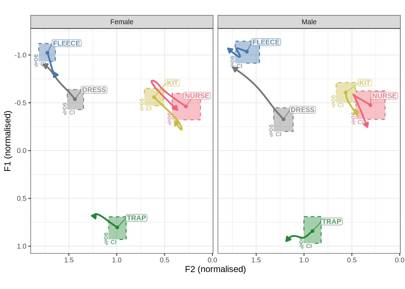
6 Plots
Having fit a models for each vowel, for both the preschoolers and the community corpus, we create plots combining the model predictions with reference information from the community and the storyteller.
6.1 Comparison plots
The first set of plots combine our models from the preschoolers and the QuakeBox models in a vowel-by-vowel ways.
comp_plot <- function(model_preds, qb_preds, vowel_name, formant_name) {

  model_preds <- model_preds %>%
    age_in_months(kids)

  caregiver_ref <- qb_preds %>%
        filter(
          generation == "Caregiver",
          vowel == vowel_name
        ) %>%
        group_by(generation) %>%
        summarise(
          caregiver_level = if_else(
            formant_name == "F1",
            mean(Predicted_F1_lob2),
            mean(Predicted_F2_lob2)
          ),
          label = "Caregiver level"
        )

  out_plot <- model_preds |>
    ggplot(
      aes(
        x = age,
        y = Predicted,
        ymin = CI_low_0.9,
        ymax = CI_high_0.9,
        colour = gender,
        fill = gender
      )
    ) +
    geom_ribbon(alpha=0.2, colour = NA) +
    geom_line(linewidth = 2) +
    geom_hline(
      aes(
        yintercept = caregiver_level,
        linetype = label
      ),
      data = caregiver_ref
    ) +
    scale_y_reverse() +
    labs(
      title = paste(vowel_name, formant_name),
      subtitle = "Model predictions QB1 vs Preschoolers (90% CI)",
      x = "Age (months)",
      y = "Normalised formant value (predicted)",
      colour = "Gender",
      fill = "Gender",
      linetype = "Reference"
    )
}

comp_plot(dress_f1_preds, QB1_preds, "DRESS", "F1") %>% print()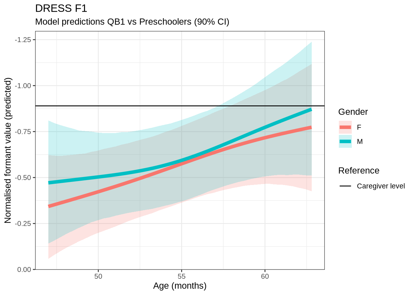
Figure 65 shows the preschoolers, both male and female, approaching the caregiver level (the black line) in dress F1.
We now apply the plot function to each of the models.
comp_plots <- expand_grid(
  vowel = c("DRESS", "FLEECE", "KIT", "NURSE", "TRAP"),
  formant_name = c("F1", "F2")
)

mod_predictions = list(
  dress_f1_preds,
  dress_f2_preds,
  fleece_f1_preds,
  fleece_f2_preds,
  kit_f1_preds,
  kit_f2_preds,
  nurse_f1_preds,
  nurse_f2_preds,
  trap_f1_preds,
  trap_f2_preds
)

comp_plots <- comp_plots |>
  mutate(
    predictions = mod_predictions
  )

comp_plots <- comp_plots |>
  mutate(
    plot = pmap(
      list(predictions, vowel, formant_name),
      \(kids_preds, v, f) {
        comp_plot(
          kids_preds,
          QB1_preds,
          v, f
        )
      }
    )
)walk(
comp_plots$plot,
print
)
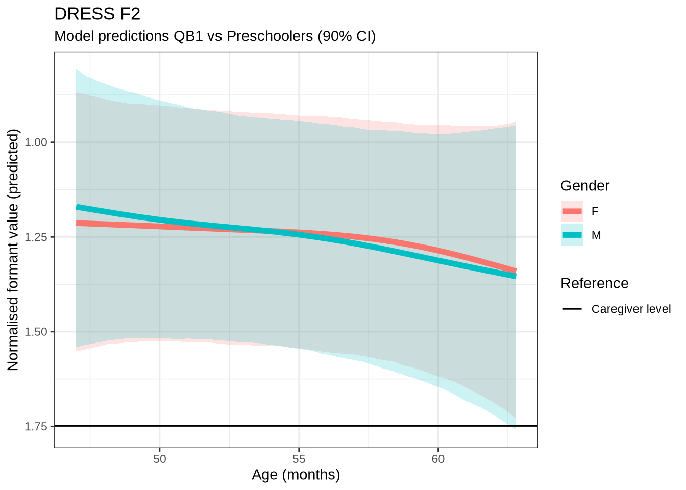
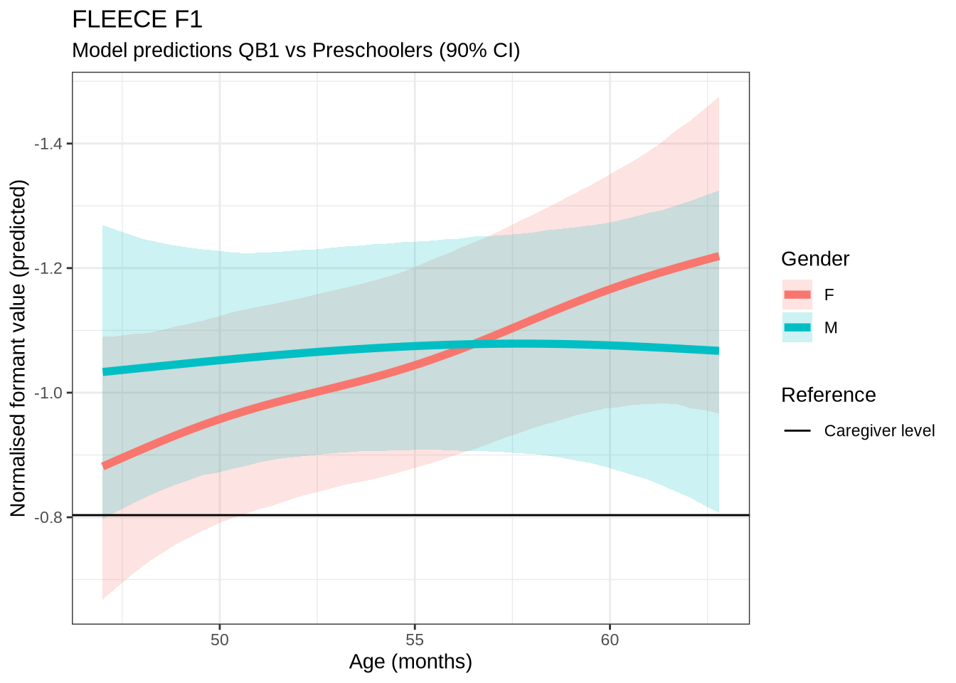
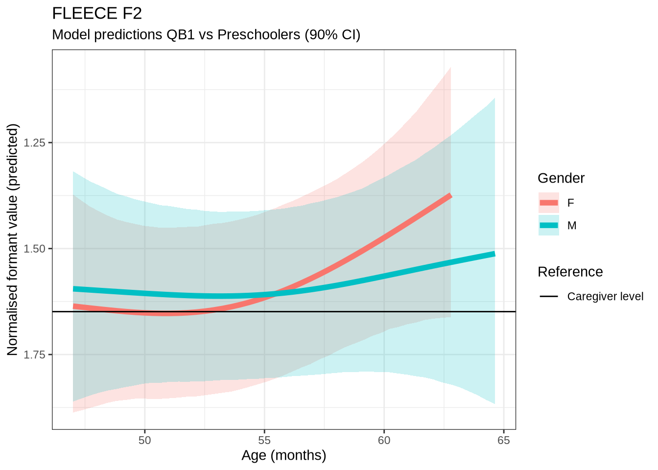
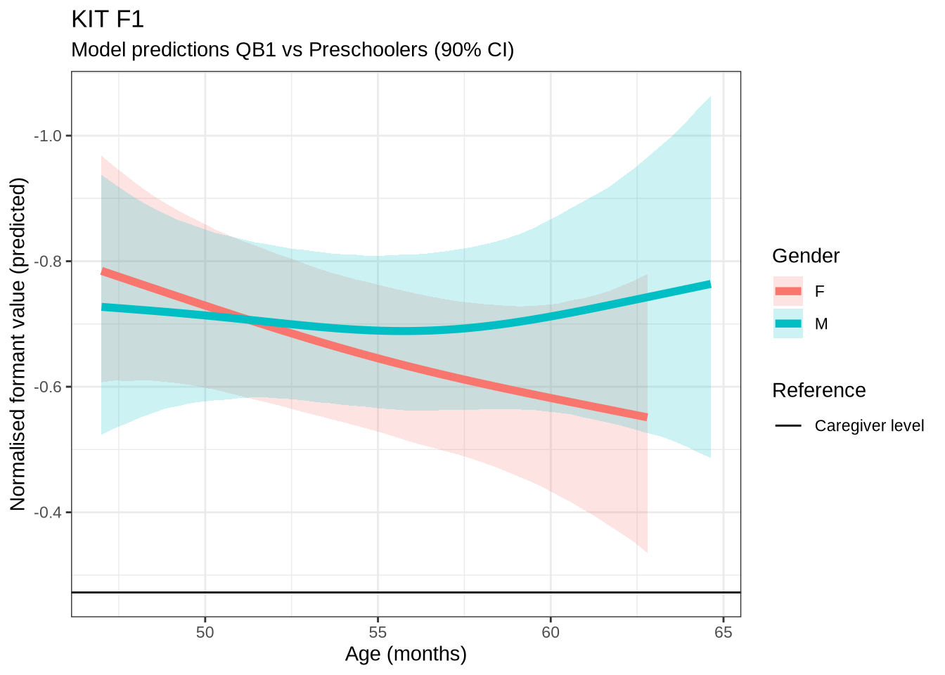
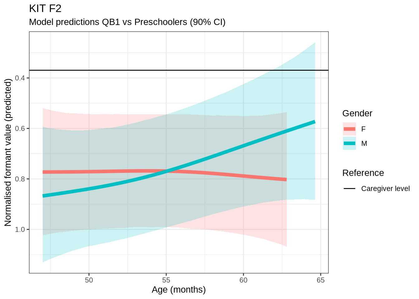
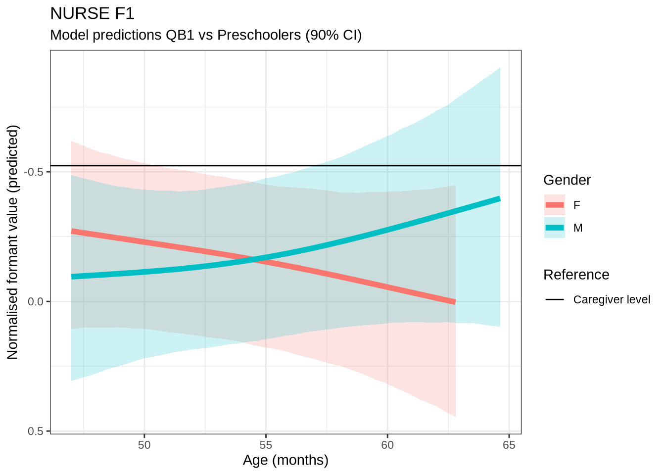
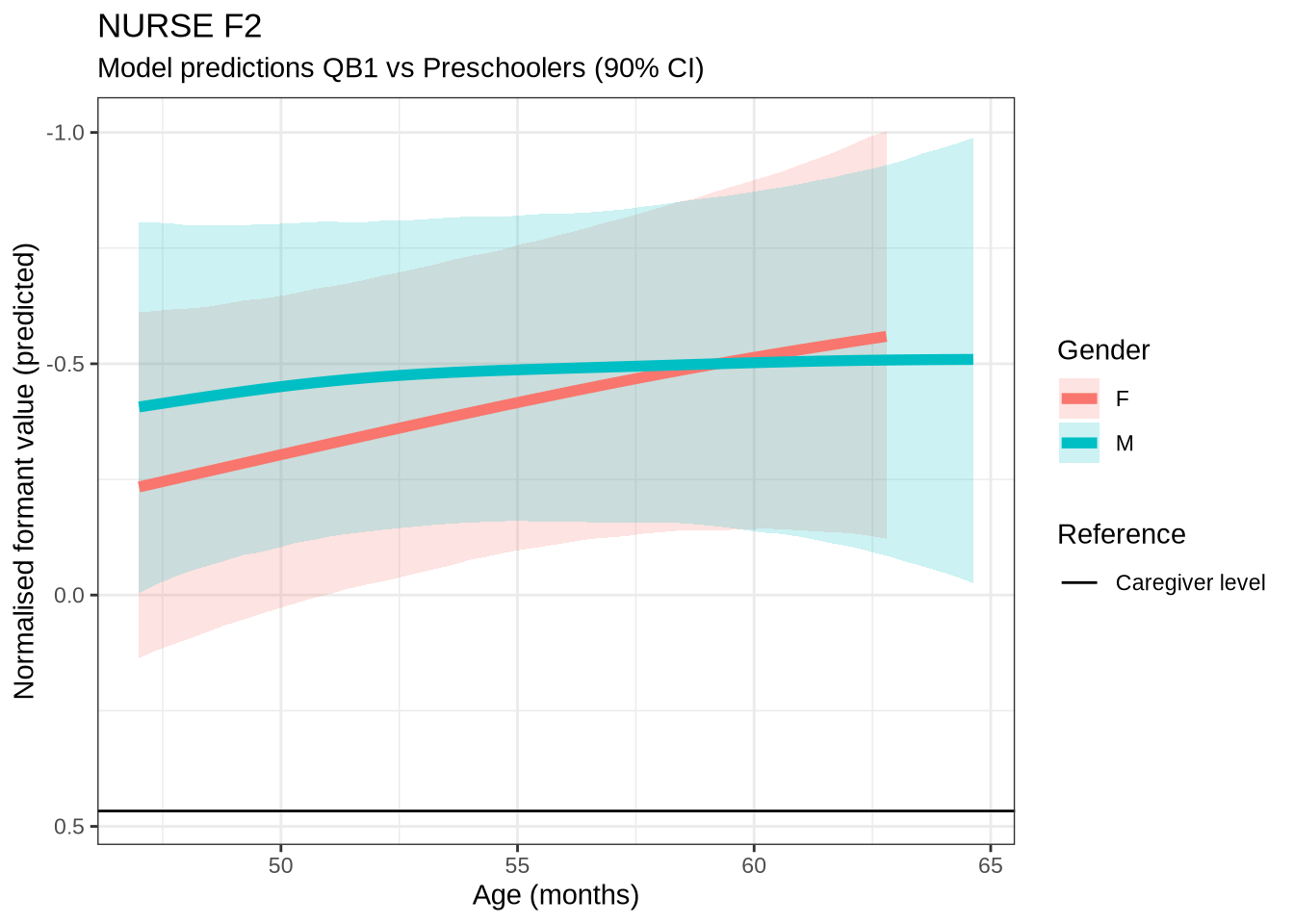
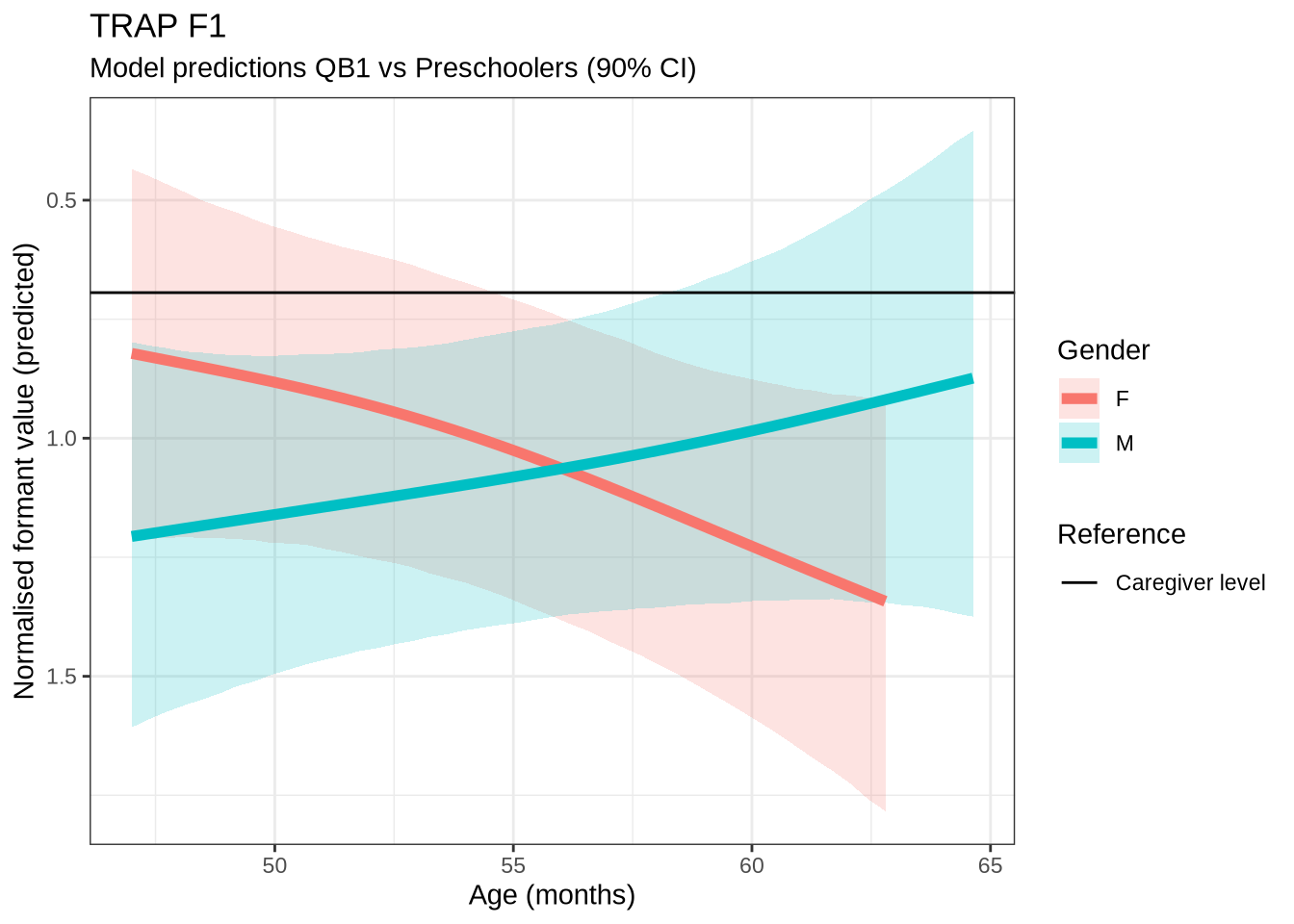
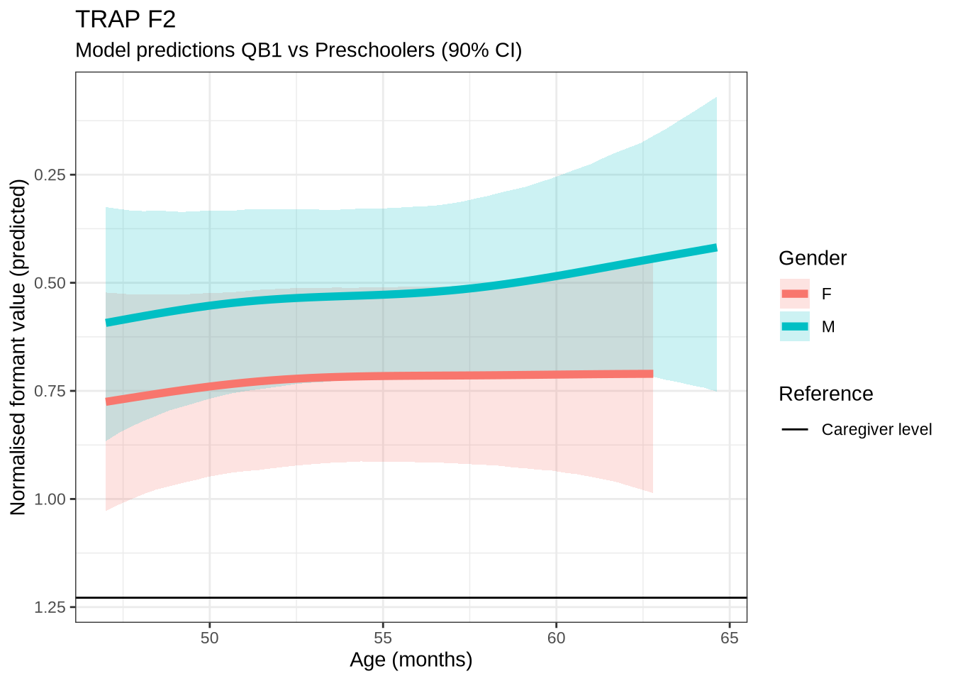
We output a figure for the paper (Figure 5) here selecting fleece F1, dress F1, kit F1 and F2.
plot_1 <- comp_plots |>
  filter(
    vowel == "FLEECE",
    formant_name == "F1"
  ) |>
  pull(plot) |>
  pluck(1) +
  labs(subtitle = NULL)

plot_2 <- comp_plots |>
  filter(
    vowel == "DRESS",
    formant_name == "F1"
  ) |>
  pull(plot) |>
  pluck(1) +
  labs(subtitle = NULL)

plot_3 <- comp_plots |>
  filter(
    vowel == "KIT",
    formant_name == "F1"
  ) |>
  pull(plot) |>
  pluck(1) +
  labs(subtitle = NULL)

plot_4 <- comp_plots |>
  filter(
    vowel == "KIT",
    formant_name == "F2"
  ) |>
  pull(plot) |>
  pluck(1) +
  labs(subtitle = NULL)

combined_plot <- (plot_1 + plot_2) /
  (plot_3 + plot_4) +
  plot_layout(guides = "collect") +
  plot_annotation(tag_levels = "A")

ggsave(
  filename = here('plots', 'figure7_combined_smooths.tiff'),
  plot = combined_plot,
  width = 14,
  height = 10,
  dpi = 300
)

combined_plot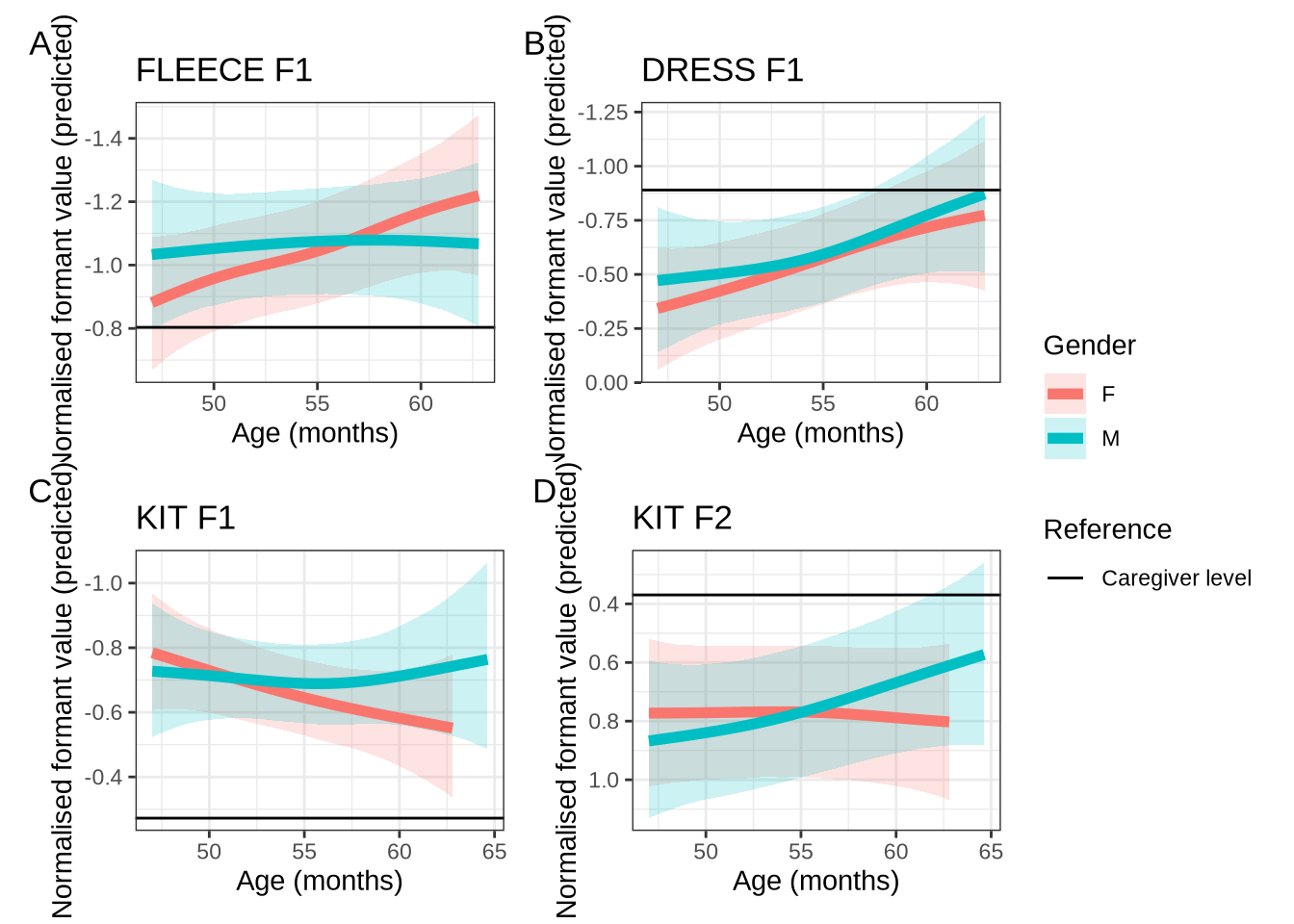
6.2 Vowel space plots
We now plot all the models in a vowel space diagram. For the paper, we restrict ourselves to the span from 50 to 60 months (i.e. 4;2 to 5). This is the main plot for the paper.
To view code click here
model_preds <- comp_plots |>
  select(vowel, formant_name, predictions) |>
  unnest(predictions)

# We widen the dataframe to get a column for F1 and for F2.
model_widepreds <- model_preds |>
  select(
    vowel, gender, age_s, formant_name, Predicted, contains("CI")
  ) %>%
  pivot_wider(
    names_from = 'formant_name',
    values_from = c('Predicted', contains("CI"))
  ) |>
  mutate(
    age = age_s * sd(kids$age) + mean(kids$age)
  ) %>%
  filter(
    between(age, 50, 60)
  )

ref_points <- QB1_preds %>%
  group_by(vowel, generation) %>%
  summarise(
    Predicted_F1 = mean(Predicted_F1_lob2),
    Predicted_F2 = mean(Predicted_F2_lob2)
  ) %>%
  mutate(
    generation = case_when(
      generation == "Oldest" ~ "Oldest adults (F)",
      generation == "Caregiver" ~ "Caregivers (F)",
      .default = generation
    )
  ) %>%
  crossing(
    gender = c("M", "F")
  ) %>%
  bind_rows(
    model_widepreds %>%
      group_by(vowel, gender) %>%
      filter(age == min(age)) %>%
      select(vowel, gender, Predicted_F1, Predicted_F2) %>%
      mutate(
        generation = "Youngest Children (4;2)"
      )
  ) %>%
  filter(
    generation != "Other",
    vowel %in% short_front
  ) %>%
  mutate(
    vowel = factor(vowel, levels = short_front),
    gender = if_else(gender == "F", "Female", "Male"),
    gender = factor(gender, levels = c("Female", "Male"))
  )

ci_boxes <- model_widepreds %>%
  group_by(vowel) %>%
  filter(
    age == min(age)
  ) %>%
  mutate(
    gender = if_else(gender == "F", "Female", "Male")
  ) %>%
  # There's probably a more compact way to do this, but this works.
  pivot_longer(
    cols = contains("CI", ignore.case = FALSE),
    names_to = "int_type",
    values_to = "int_value"
  ) %>%
  mutate(
    # Get values of form "CI_height_formant
    which_side = str_replace_all(int_type, "_0.[79]", ""),
    # Get size of credibile interval
    which_size = str_extract(int_type, "0.[79]")
  ) %>%
  select(-int_type) %>%
  pivot_wider(
    names_from = which_side,
    values_from = int_value
  ) %>%
  group_by(vowel, gender, which_size) %>%
  nest() %>%
  mutate(
    cis = map(
      data,
      ~ {
        points <- .x %>%
          select(
            CI_high_F2, CI_low_F2,
            CI_high_F1, CI_low_F1
          ) %>%
          pivot_longer(
            cols = everything(),
            names_to = "type",
            values_to = "value"
          ) %>%
          mutate(
            formant = str_extract(type, "F[1-2]")
          ) %>%
          select(formant, value)
        out <- crossing(
          "F1" = points %>%
            filter(formant == "F1") %>%
            pull(value),
          "F2" = points %>%
            filter(formant == "F2") %>%
            pull(value)
        )
        out %>%
          # order correctly for polygon.
          slice(c(1, 2, 4, 3, 1))
      }
    )
  ) %>%
  select(-data) %>%
  unnest(cis) %>%
  filter(
    vowel %in% short_front
  ) %>%
  mutate(
    label = if_else(which_size == 0.7, "70% CI", "90% CI"),
    vowel_group = str_c(vowel, label)
  )

kids_plot <- model_widepreds %>%
  group_by(vowel, gender) %>%
  mutate(
    label = if_else(age == min(age), vowel, "")
  ) %>%
  ungroup() %>%
  mutate(
    vowel = factor(vowel, levels = short_front),
    gender = if_else(gender == "F", "Female", "Male"),
    gender = factor(gender, levels = c("Female", "Male"))
  ) %>%
  ggplot(
    aes(
      x = Predicted_F2,
      y = Predicted_F1,
      colour = vowel
    )
  ) +
  geom_path(
    show.legend = FALSE,
    arrow = arrow(
        ends = "last",
        type="closed",
        length = unit(2, "mm")
      ),
    linetype = 1,
    linewidth = 0.7
  ) +
  geom_textpath(
    aes(
      x = F2,
      y = F1,
      colour = vowel,
      label = label,
      group = vowel_group
    ),
    linetype = "dashed",
    vjust = 1,
    size = 1.5,
    inherit.aes = FALSE,
    data = ci_boxes
  ) +
  geom_polygon(
    aes(
      x = F2,
      y = F1,
      fill = vowel,
      group = vowel_group
    ),
    linewidth = 0,
    alpha = 0.2,
    inherit.aes = FALSE,
    data = ci_boxes
  ) +
  geom_label_repel(
    aes(label = label),
    size = 2,
    max.overlaps = 50,
    label.padding = 0.1,
    fontface = "bold",
    alpha = 0.8,
    #nudge_x = 0.2,
    #nudge_y = 0.1,
    min.segment.length = 0
    ) +
  geom_point(aes(shape = generation), size = 3, data = ref_points) +
  scale_x_reverse(expand = expansion(mult = 0.1)) +
  scale_y_reverse() +
  scale_colour_manual(values = vowel_colours_5) +
  scale_fill_manual(values = vowel_colours_5) +
  coord_fixed() +
  scale_shape_manual(
    values = list(
      "Caregivers (F)" = 18,
      "Youngest Children (4;2)" = 20,
      "Oldest adults (F)" = 4
    )
  ) +
  labs(
    y = "F1 (normalised)",
    x = "F2 (normalised)",
    colour = "Vowel",
    shape = "Population"
  ) +
  guides(
    color = "none",
    fill = "none"
  ) +
  facet_grid(cols = vars(gender)) +
  theme(
    legend.position = "bottom"
  )

ggsave(
  here('plots', 'figure5_model_preds.tiff'),
  plot = kids_plot,
  width = 8,
  height = 5,
  dpi = 500
)

kids_plot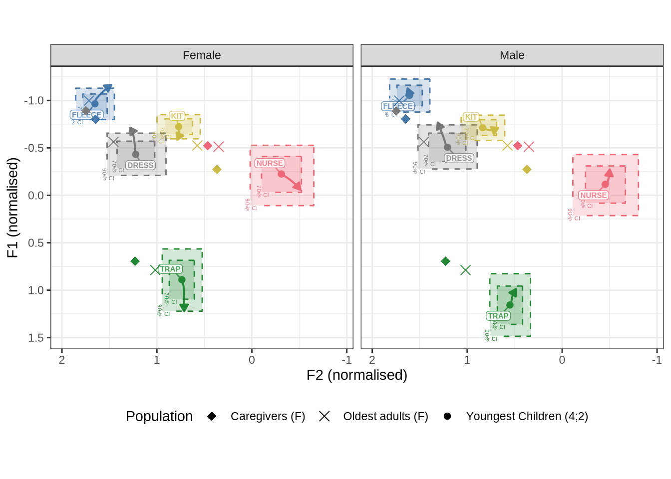
We now add the story teller and some vowel space triangles.
storyteller_means <- read_rds(here('data', 'storyteller_means.rds'))

storyteller_means <- storyteller_means |>
  rename(
    vowel = celex_vowel,
    Predicted_F1 = F1_lob2,
    Predicted_F2 = F2_lob2
  ) |>
  mutate(
    generation = "Storyteller (M)"
  ) |>
  filter(
    vowel %in% short_front
  ) %>%
  crossing(
    gender = c("Male", "Female")
  )

ref_points <- ref_points %>%
  bind_rows(storyteller_means)

group_paths <- ref_points %>%
  filter(
    gender == "Female",
    vowel %in% c("NURSE", "FLEECE", "TRAP"),
    generation != "Oldest adults (F)"
  ) %>%
  arrange(vowel)

out_plot <- model_widepreds %>%
  filter(
    gender == "F"
  ) %>%
  mutate(
    vowel = factor(vowel, levels = short_front)
  ) %>%
  ggplot(
    aes(
      x = Predicted_F2,
      y = Predicted_F1,
      colour = vowel
    )
  ) +
  geom_path(
    show.legend = FALSE,
    arrow = arrow(
        ends = "last",
        type="closed",
        length = unit(2, "mm")
      ),
    linetype = 1,
    linewidth = 0.7
  ) +
  geom_point(aes(shape = generation), data = ref_points, size = 4) +
  geom_polygon(
    aes(
      linetype = generation
    ),
    linewidth = 1,
    colour = "black",
    fill = "NA",
    data = group_paths
  ) +
  scale_x_reverse(expand = expansion(mult = 0.1), position = "top") +
  scale_y_reverse(position = "right") +
  scale_colour_manual(values = vowel_colours_5) +
  scale_shape_manual(
    values = list(
      "Caregivers (F)" = 18,
      "Youngest Children (4;2)" = 20,
      "Oldest adults (F)" = 4,
      "Storyteller (M)" = 7
    )
  ) +
  coord_fixed() +
  labs(
    y = "F1 (normalised)",
    x = "F2 (normalised)",
    colour = "Vowel",
    shape = "Population (Points)",
    linetype = "Population (Triangle)"
  ) +
  guides(
    color = guide_legend(
      override.aes = list(fill=NA),
      order = 3
    ),
    shape = guide_legend(order = 4)
  )

ggsave(
  here('plots', 'figure9_storyteller.tiff'),
  plot = out_plot,
  width = 7,
  height = 5,
  dpi = 500
)

out_plot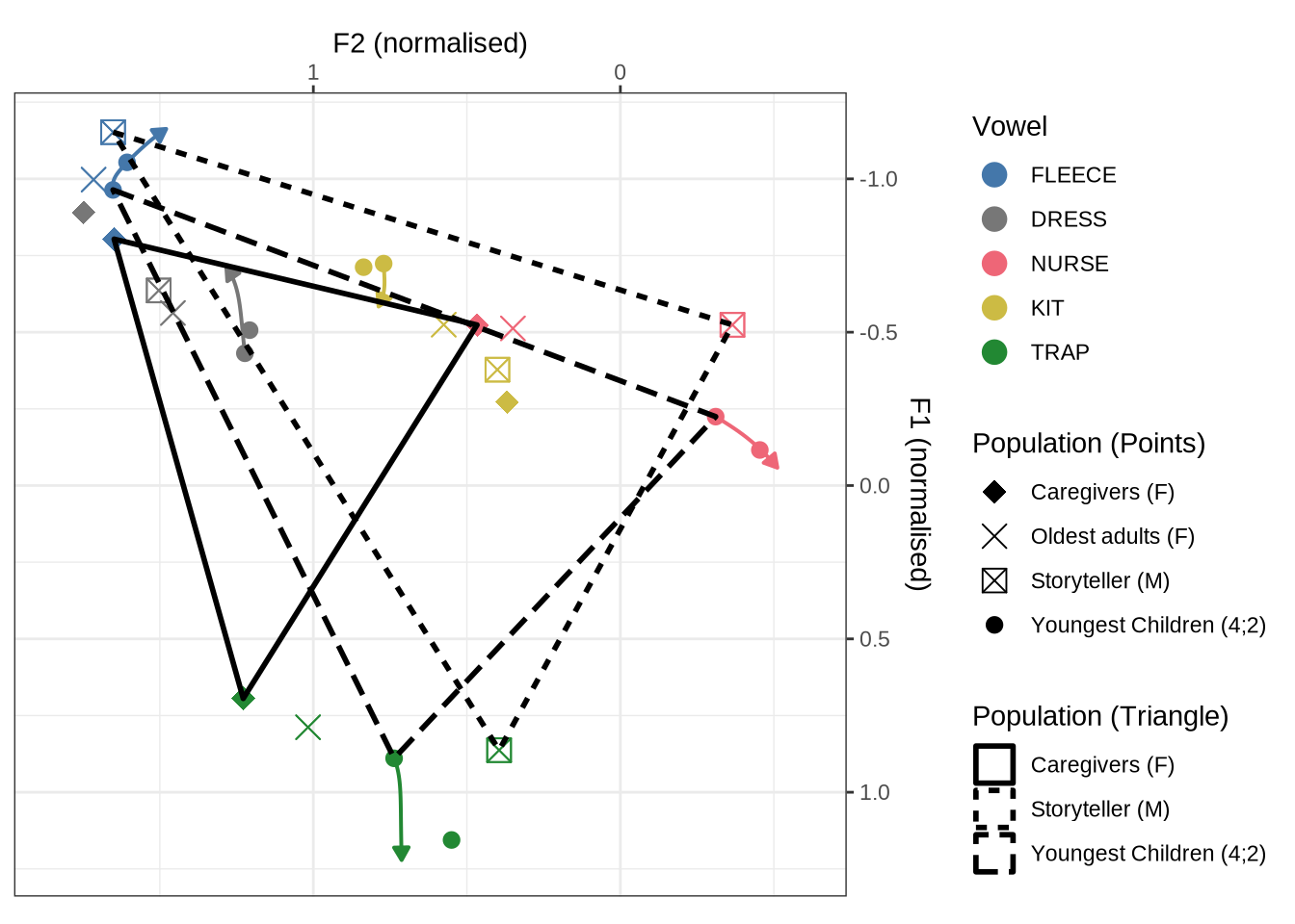
7 Additional tests
7.1 Longitudinal models
Each model, applied to the preschoolers, has already been compared with the data viewed longitudinally, with mixed results (e.g. Figure 7).
But let’s try a modelling approach which foregrounds the longitudinal nature of the data. This one will use ‘collect’ as the primary explanatory variable rather than age. This provides another way to approach the data longitudinally, which we can compare with the results presented above.
We’ll just do this for the four variables highlighted in Figure 66.
7.1.1 dress F1
# Create dataframe for F1 models
f1 <- kids |>
  filter(!F1_outlier) |>
  select(
    participant, collect, age_s, gender, word, vowel, stressed, stopword,
    F1_lob2, duration_s, age
  ) |>
  mutate(
    gender = as.factor(gender),
    word = as.factor(word)
  )

dress_f1_data <- f1 |>
  filter(
    vowel == "DRESS"
  ) |>
  mutate(
    w_s = interaction(word, stressed),
    p_c = interaction(participant, collect)
  ) %>%
  droplevels()
Let’s have a look at the data first.
collect_plot <- function(vowel_data, formant="F1") {
  vowel_data %>%
    group_by(participant) %>%
    mutate(
      n_collects = n_distinct(collect)
    ) %>%
    filter(
      n_collects > 2
    ) %>%
    group_by(participant, collect) %>%
    summarise(
      formant = mean(.data[[paste0(formant, "_lob2")]]),
      gender = first(gender)
    ) %>%
    ggplot(
      aes(
        y = formant,
        x = collect,
        colour = gender,
        group = participant
      )
    ) +
    geom_point() +
    geom_path() +
    scale_y_reverse()
}

collect_plot(dress_f1_data)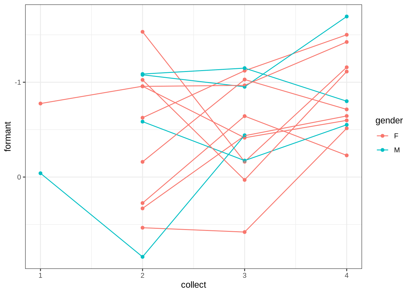
Figure 69 suggests a wide range of values at collection point two, tightening at three, and then raising (in the vowel space) at point four.
summary(dress_f1_data) participant collect age_s gender word
Length:945 Min. :1.000 Min. :-1.83828 F:531 then :475
Class :character 1st Qu.:2.000 1st Qu.:-0.84298 M:414 went : 80
Mode :character Median :3.000 Median :-0.09651 said : 77
Mean :2.666 Mean :-0.08124 nest : 44
3rd Qu.:4.000 3rd Qu.: 0.64996 better : 31
Max. :4.000 Max. : 2.14290 remember: 27
(Other) :211
vowel stressed stopword F1_lob2
DRESS:945 Mode :logical Mode :logical Min. :-3.6074
FALSE:36 FALSE:356 1st Qu.:-1.1944
TRUE :909 TRUE :589 Median :-0.7474
Mean :-0.5646
3rd Qu.:-0.0281
Max. : 4.3793
duration_s age w_s p_c
Min. :-0.8999 Min. :47.00 then.TRUE :457 EC0919-Child.1: 23
1st Qu.:-0.5655 1st Qu.:51.00 went.TRUE : 80 EC0105-Child.2: 22
Median :-0.2499 Median :54.00 said.TRUE : 74 EC2432-Child.3: 20
Mean :-0.1059 Mean :54.06 nest.TRUE : 44 EC0503-Child.2: 19
3rd Qu.: 0.1844 3rd Qu.:57.00 better.TRUE : 29 EC0501-Child.2: 18
Max. : 2.4698 Max. :63.00 remember.TRUE: 26 EC0501-Child.1: 17
(Other) :235 (Other) :826 Let’s model it. We replace year of birth with collection point in the model structure from last time, with random intercepts for each participant and collect, which should in theory help to control for chronological age.
dress_f1_fit <- brm(
    F1_lob2 ~ stopword + factor(collect) * gender +
      duration_s +
      (1 | w_s) +
      (1 | p_c),
    data = dress_f1_data,
    family = student(),
    chains = 4,
    cores = 4,
    iter = 3000,
    control = list(adapt_delta = 0.9),
  )

write_rds(dress_f1_fit, here('models', 'dress_F1_long.rds'))
We estimate the change over time at the collect level.
estimate_relation(
  dress_f1_fit,
  by = c("collect", "gender"),
  allow_new_levels = TRUE,
  ci = 0.90,
) %>%
  plot() +
  scale_y_reverse()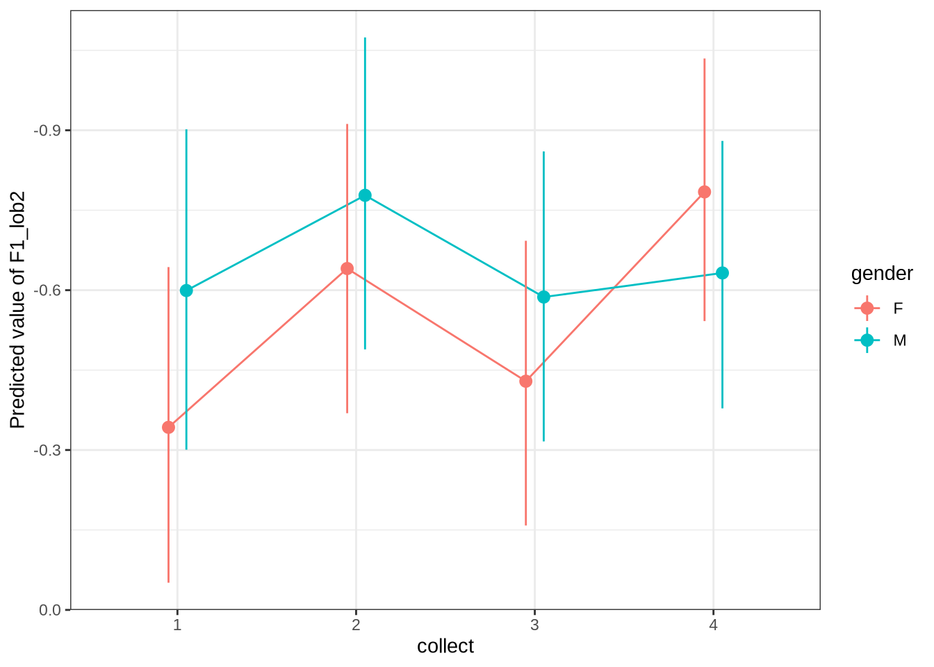
Figure 70 suggests rising in the vowel space for female preschoolers between collection points three and four, but nothing much else. This is more-or-less consistent with our age based model for the female preschoolers. The across-the-board rising in the vowel space we see for males is not borne out. But there are only four male preschoolers here, so this should not worry us massively.
7.1.2 fleece F1
Let’s look at [fleece] F1.
fleece_f1_data <- f1 |>
  filter(
    vowel == "FLEECE"
  ) |>
  mutate(
    w_s = interaction(word, stressed),
    p_c = interaction(participant, collect)
  ) %>%
  droplevels()

collect_plot(fleece_f1_data)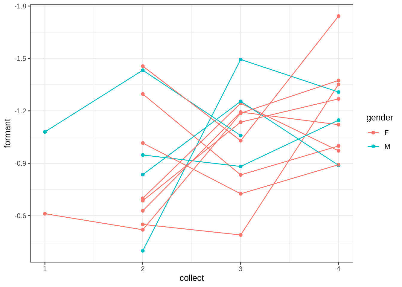
Figure 71 is a similar story to Figure 69. Some kind of stability between two and three and an increase at four. Note also that the three of the males start very low in the vowel space at time two then increase at time three.
summary(fleece_f1_data) participant collect age_s gender word
Length:1116 Min. :1.000 Min. :-1.83828 F:595 he :440
Class :character 1st Qu.:2.000 1st Qu.:-0.84298 M:521 the :189
Mode :character Median :3.000 Median :-0.09651 she :174
Mean :2.849 Mean : 0.01162 tui : 65
3rd Qu.:4.000 3rd Qu.: 0.64996 he's : 34
Max. :4.000 Max. : 2.14290 see : 29
(Other):185
vowel stressed stopword F1_lob2
FLEECE:1116 Mode :logical Mode :logical Min. :-3.7569
FALSE:129 FALSE:238 1st Qu.:-1.5829
TRUE :987 TRUE :878 Median :-1.1389
Mean :-1.0330
3rd Qu.:-0.5608
Max. : 3.6886
duration_s age w_s p_c
Min. :-1.0124 Min. :47.00 he.TRUE :427 EC0405-Child.2: 24
1st Qu.:-0.6548 1st Qu.:51.00 the.TRUE :181 EC1522-Child.1: 19
Median :-0.2972 Median :54.00 she.TRUE :171 EC0413-Child.3: 18
Mean :-0.1098 Mean :54.43 tui.FALSE: 65 EC2432-Child.3: 17
3rd Qu.: 0.2392 3rd Qu.:57.00 he's.TRUE: 33 EC0914-Child.4: 17
Max. : 2.3906 Max. :63.00 see.TRUE : 28 EC1106-Child.4: 17
(Other) :211 (Other) :1004 Let’s model.
fleece_f1_fit <- brm(
    F1_lob2 ~ stopword + factor(collect) * gender +
      duration_s +
      (1 | w_s) +
      (1 | p_c),
    data = fleece_f1_data,
    family = student(),
    chains = 4,
    cores = 4,
    iter = 3000,
    control = list(adapt_delta = 0.9),
  )


write_rds(fleece_f1_fit, here('models', 'fleece_F1_long.rds'))estimate_relation(
fleece_f1_fit,
by = c("collect", "gender"),
allow_new_levels = TRUE,
ci = 0.9
) %>%
plot() +
scale_y_reverse()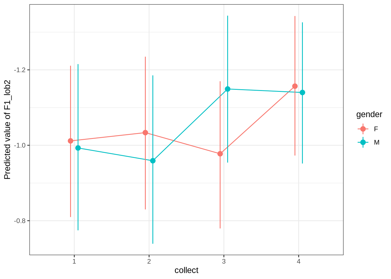
The apparent raising in the vowel space occurs where expected for both genders. However, with out 90% credible intervals, there’s no obvious place where we the mean value at one collect is outside the 90% credible interval for the next collection point. Nonetheless, the pattern of raising towards the end is at least consistent with out age-based models.
7.1.3 kit F1
Time for kit.
fleece_f1_data <- f1 |>
  filter(
    vowel == "KIT"
  ) |>
  mutate(
    w_s = interaction(word, stressed),
    p_c = interaction(participant, collect)
  ) %>%
  droplevels()

collect_plot(kit_f1_data)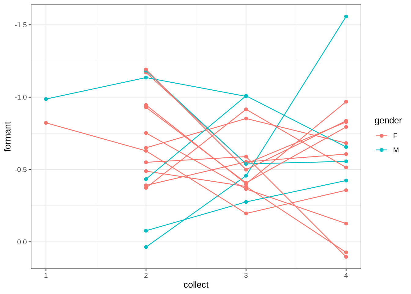
Maybe kit F1 is showing a lowering in the vowel space for the female preschoolers. There’s nothing obvious happening for the male preschoolers.
summary(kit_f1_data) participant collect age_s gender word
Length:1837 Min. :1.000 Min. :-1.83828 F:975 his : 211
Class :character 1st Qu.:2.000 1st Qu.:-0.84298 M:862 him : 190
Mode :character Median :3.000 Median : 0.15231 it : 112
Mean :2.801 Mean : 0.05966 bridge : 90
3rd Qu.:4.000 3rd Qu.: 0.89878 the : 87
Max. :4.000 Max. : 2.64055 baby : 65
(Other):1082
vowel stressed stopword F1_lob2
KIT:1837 Mode :logical Mode :logical Min. :-3.57123
FALSE:652 FALSE:1047 1st Qu.:-1.20097
TRUE :1185 TRUE :790 Median :-0.62589
Mean :-0.55152
3rd Qu.: 0.06089
Max. : 5.35072
duration_s age w_s p_c
Min. :-0.8373 Min. :47.00 his.TRUE : 202 EC1402-Child.3: 38
1st Qu.:-0.5859 1st Qu.:51.00 him.TRUE : 175 EC0405-Child.2: 30
Median :-0.2749 Median :55.00 it.TRUE : 109 EC0918-Child.4: 27
Mean :-0.0985 Mean :54.63 bridge.TRUE: 88 EC0901-Child.4: 24
3rd Qu.: 0.1750 3rd Qu.:58.00 the.TRUE : 87 EC0102-Child.4: 23
Max. : 2.4875 Max. :65.00 baby.FALSE : 65 EC2024-Child.1: 22
(Other) :1111 (Other) :1673 Let’s model.
kit_f1_fit <- brm(
    F1_lob2 ~ stopword + factor(collect) * gender +
      duration_s +
      (1 | w_s) +
      (1 | p_c),
    data = kit_f1_data,
    family = student(),
    chains = 4,
    cores = 4,
    iter = 3000,
    control = list(adapt_delta = 0.9),
  )


write_rds(kit_f1_fit, here('models', 'kit_F1_long.rds'))estimate_relation(
kit_f1_fit,
by = c("collect", "gender"),
allow_new_levels = TRUE,
ci = 0.9
) %>%
plot() +
scale_y_reverse()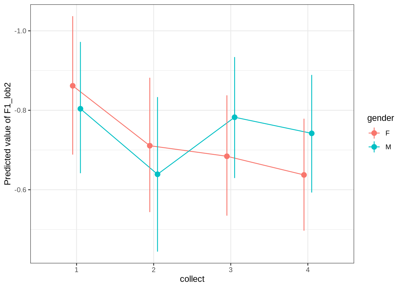
The broad pattern in Figure 74 is a small lowering in the vowel space for female preschoolers and no clear pattern in the males. This is broadly consistent with the patterns identified in the age-based models.
7.1.4 kit F2
f2 <- kids |>
  filter(!F2_outlier) |>
  select(
    participant, collect, age_s, gender, word, vowel, stressed, stopword,
    F2_lob2, duration_s, age
  ) |>
  mutate(
    gender = as.factor(gender),
    word = as.factor(word)
  )

kit_f2_data <- f2 |>
  filter(
    vowel == "KIT"
  ) |>
  mutate(
    w_s = interaction(word, stressed),
    p_c = interaction(participant, collect)
  ) %>%
  droplevels()

collect_plot(kit_f2_data, formant = "F2")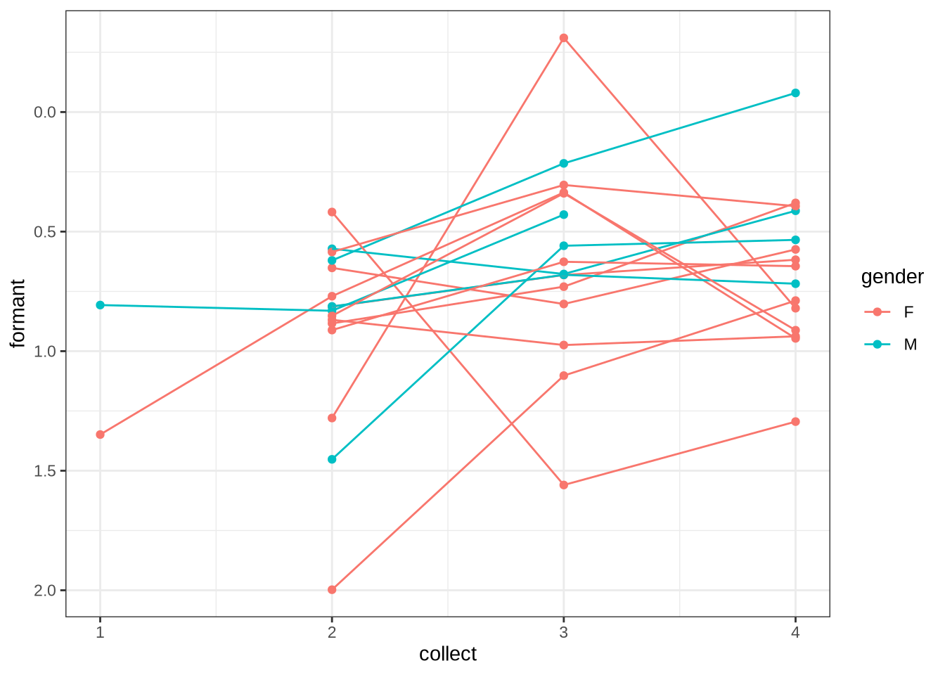
Figure 75 suggests backing for male preschoolers, and some kind of tighter clustering for female preschoolers by the time they hit collection point four.
summary(kit_f2_data) participant collect age_s gender word
Length:1801 Min. :1.00 Min. :-1.83828 F:952 his : 205
Class :character 1st Qu.:2.00 1st Qu.:-0.84298 M:849 him : 193
Mode :character Median :3.00 Median : 0.15231 it : 115
Mean :2.79 Mean : 0.05726 bridge : 89
3rd Qu.:4.00 3rd Qu.: 0.89878 the : 88
Max. :4.00 Max. : 2.64055 baby : 62
(Other):1049
vowel stressed stopword F2_lob2
KIT:1801 Mode :logical Mode :logical Min. :-1.6722
FALSE:623 FALSE:1007 1st Qu.: 0.2130
TRUE :1178 TRUE :794 Median : 0.7956
Mean : 0.7546
3rd Qu.: 1.3374
Max. : 3.5166
duration_s age w_s p_c
Min. :-0.83729 Min. :47.00 his.TRUE : 196 EC1402-Child.3: 35
1st Qu.:-0.58349 1st Qu.:51.00 him.TRUE : 178 EC0405-Child.2: 30
Median :-0.27489 Median :55.00 it.TRUE : 112 EC0918-Child.4: 28
Mean :-0.09937 Mean :54.62 the.TRUE : 88 EC0102-Child.4: 23
3rd Qu.: 0.17504 3rd Qu.:58.00 bridge.TRUE: 87 EC0901-Child.4: 23
Max. : 2.48745 Max. :65.00 baby.FALSE : 62 EC0501-Child.1: 21
(Other) :1078 (Other) :1641 We’ll model this.
kit_f2_fit <- brm(
    F2_lob2 ~ stopword + factor(collect) * gender +
      duration_s +
      (1 | w_s) +
      (1 | p_c),
    data = kit_f2_data,
    family = student(),
    chains = 4,
    cores = 4,
    iter = 3000,
    control = list(adapt_delta = 0.9),
  )


write_rds(kit_f2_fit, here('models', 'kit_F2_long.rds'))estimate_relation(
kit_f2_fit,
by = c("collect", "gender"),
allow_new_levels = TRUE,
ci = 0.9
) %>%
plot() +
scale_y_reverse()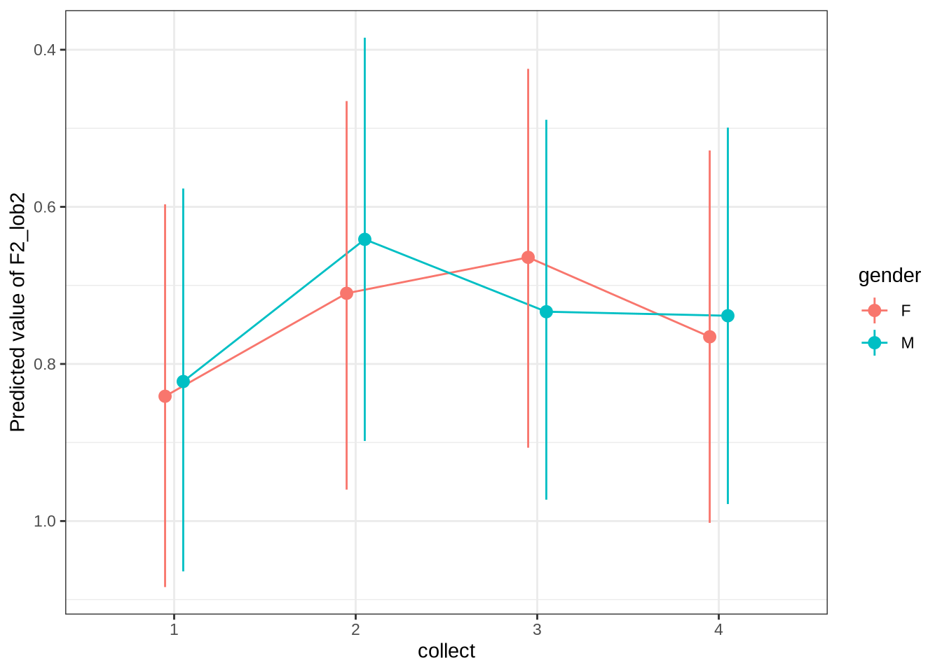
Interestingly, Figure 76 does not seem to match the backing story we had for male speakers. In both cases, there’s nothing obvious going on.
7.2 Non-imputed analysis
We now model with the non-imputed version of Lobanov 2.0. The point of this is to get some indication that the imputation of values carried out as part of our normalisation process did not bias our results.
Note that nurse is not in the top-5 vowel types, so cannot be modelled here.
Again, we’re just looking for broad agreement with our existing models which include the imputed data.
f1 <- kids |>
  filter(!F1_outlier) |>
  select(
    participant, collect, age_s, gender, word, vowel, stressed, stopword,
    F1_sub, age, duration_s
  ) |>
  mutate(
    gender = as.factor(gender),
    word = as.factor(word)
  )

f2 <- kids |>
  filter(!F2_outlier) |>
  select(
    participant, collect, age_s, gender, word, vowel, stressed, stopword,
    F2_sub, age, duration_s
  ) |>
  mutate(
    gender = as.factor(gender),
    word = as.factor(word)
  )
7.2.1 dress F1
dress_f1_data <- f1 |>
  filter(
    vowel == "DRESS"
  ) |>
  mutate(
    w_s = interaction(word, stressed),
    p_c = interaction(participant, collect)
  ) %>%
  droplevels() %>%
  filter(
    !is.na(F1_sub)
)summary(dress_f1_data) participant collect age_s gender word
Length:571 Min. :1.000 Min. :-1.83828 F:342 then :310
Class :character 1st Qu.:2.000 1st Qu.:-0.84298 M:229 said : 50
Mode :character Median :3.000 Median :-0.09651 went : 47
Mean :2.795 Mean :-0.06514 nest : 23
3rd Qu.:4.000 3rd Qu.: 0.64996 better : 21
Max. :4.000 Max. : 2.14290 again : 12
(Other):108
vowel stressed stopword F1_sub age
DRESS:571 Mode :logical Mode :logical Min. :-5.50648 Min. :47.00
FALSE:27 FALSE:197 1st Qu.:-1.11561 1st Qu.:51.00
TRUE :544 TRUE :374 Median :-0.62002 Median :54.00
Mean :-0.51046 Mean :54.13
3rd Qu.: 0.01216 3rd Qu.:57.00
Max. : 4.69020 Max. :63.00
duration_s w_s p_c
Min. :-0.89992 then.TRUE :293 EC0919-Child.1: 23
1st Qu.:-0.53849 said.TRUE : 49 EC2432-Child.3: 20
Median :-0.22038 went.TRUE : 47 EC0503-Child.2: 19
Mean :-0.09484 nest.TRUE : 23 EC0501-Child.2: 18
3rd Qu.: 0.18437 better.TRUE: 19 EC0501-Child.1: 17
Max. : 2.46981 then.FALSE : 17 EC2432-Child.2: 15
(Other) :123 (Other) :459 dress_f1_fit_sub <- brm(
F1_sub ~ gender + stopword +
s(age_s, by=gender, k = 5) +
s(duration_s, k = 5) +
(1 | w_s) +
(1 | p_c),
data = dress_f1_data,
family = student(),
prior = prior_t,
chains = 4,
cores = 4,
iter = 3000,
control = list(adapt_delta = 0.95),
)
write_rds(
dress_f1_fit_sub,
here('models', 'dress_f1_fit_sub.rds'),
compress = "gz"
)Let’s look at some model predictions.
dress_f1_preds <- estimate_relation(
    dress_f1_fit_sub,
    by = list(
      age_s = seq(min_age_s, max_age_s, length = 50),
      gender = c("F", "M"),
      duration_s = 0
    ),
    predict="link",
    ci = 0.9
  )

dress_f1_preds %>%
  plot() +
  scale_y_reverse()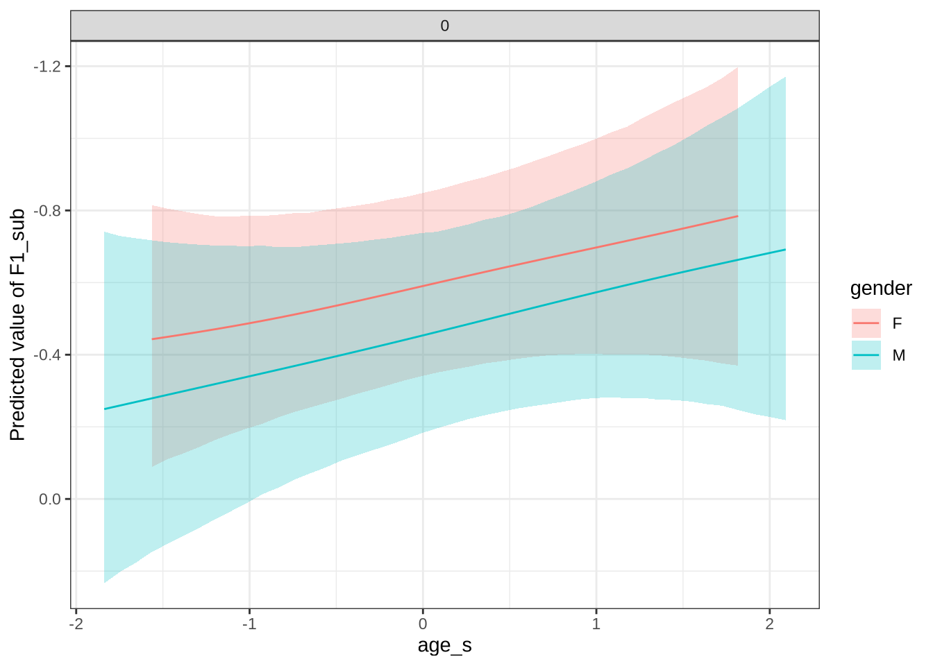
We get a broadly similar pattern to our models with imputed data (Figure 10). The vowel is going up in the vowel space. We cannot directly compare the normalised formant values with those of the community or the imputed preschooler values as they are normalised with a different vowel set.
7.2.2 fleece F1
fleece_f1_data <- f1 |>
  filter(
    vowel == "FLEECE"
  ) |>
  mutate(
    w_s = interaction(word, stressed),
    p_c = interaction(participant, collect)
  ) %>%
  droplevels()|>
  filter(
    !is.na(F1_sub)
)summary(fleece_f1_data) participant collect age_s gender word
Length:567 Min. :1.000 Min. :-1.83828 F:314 he :240
Class :character 1st Qu.:2.000 1st Qu.:-0.84298 M:253 the : 96
Mode :character Median :3.000 Median : 0.15231 she : 80
Mean :2.982 Mean : 0.07508 tui : 28
3rd Qu.:4.000 3rd Qu.: 0.89878 see : 20
Max. :4.000 Max. : 2.14290 kiwi : 16
(Other): 87
vowel stressed stopword F1_sub age
FLEECE:567 Mode :logical Mode :logical Min. :-3.5475 Min. :47.00
FALSE:74 FALSE:123 1st Qu.:-1.5641 1st Qu.:51.00
TRUE :493 TRUE :444 Median :-1.1003 Median :55.00
Mean :-1.0348 Mean :54.69
3rd Qu.:-0.5869 3rd Qu.:58.00
Max. : 3.0156 Max. :63.00
duration_s w_s p_c
Min. :-1.0124 he.TRUE :228 EC0405-Child.2: 24
1st Qu.:-0.6548 the.TRUE : 90 EC1522-Child.1: 19
Median :-0.2972 she.TRUE : 79 EC0413-Child.3: 18
Mean :-0.1248 tui.FALSE: 28 EC2432-Child.3: 17
3rd Qu.: 0.1580 see.TRUE : 20 EC0914-Child.4: 17
Max. : 2.3906 he.FALSE : 12 EC1106-Child.4: 17
(Other) :110 (Other) :455 fleece_f1_fit_sub <- brm(
F1_sub ~ gender + stopword +
s(age_s, by=gender, k = 5) +
s(duration_s, k = 5) +
(1 | w_s) +
(1 | p_c),
data = fleece_f1_data,
family = student(),
prior = prior_t,
chains = 4,
cores = 4,
iter = 3000,
control = list(adapt_delta = 0.95),
)
write_rds(
fleece_f1_fit_sub,
here('models', 'fleece_f1_fit_sub.rds'),
compress = "gz"
)Let’s look at some model predictions.
fleece_f1_preds <- estimate_relation(
    fleece_f1_fit_sub,
    by = list(
      age_s = seq(min_age_s, max_age_s, length = 50),
      gender = c("F", "M"),
      duration_s = 0
    ),
    predict="link",
    ci = 0.9
  )

fleece_f1_preds %>%
  plot() +
  scale_y_reverse()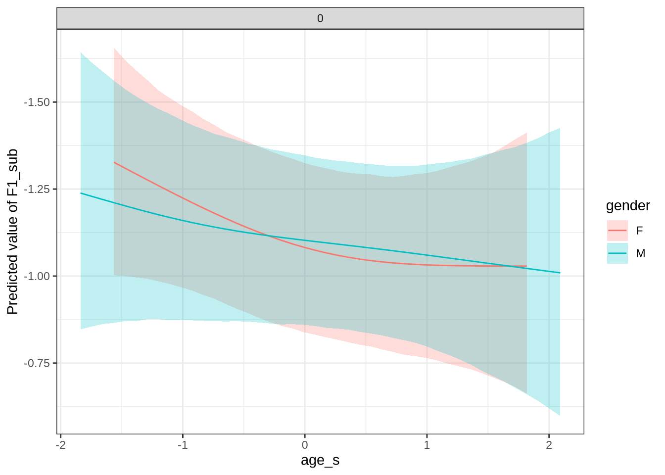
Figure 78 is much more alarming for our overall story, and is referenced in the paper. If anything, the vowel lowers in the vowel space for both male and female preschoolers, although not by much and with very wide 90% credible intervals. There are a few factors which could explain the discrepancy. We have not carried out a detailed study of normalisation with only five vowels, for instance. On the other hand, our imputation method should not bias us in the direction of move movement with age. We leave this here as warning against over interpreting the apparent extreme movements in fleece in the models reported above.
7.2.3 kit F1
We copy the above steps for kit
kit_f1_data <- f1 |>
  filter(
    vowel == "KIT"
  ) |>
  mutate(
    w_s = interaction(word, stressed),
    p_c = interaction(participant, collect)
  ) %>%
  droplevels() |>
  filter(
    !is.na(F1_sub)
)summary(kit_f1_data) participant collect age_s gender word
Length:871 Min. :1.00 Min. :-1.8383 F:488 his :118
Class :character 1st Qu.:2.00 1st Qu.:-0.5942 M:383 him : 89
Mode :character Median :3.00 Median : 0.1523 it : 58
Mean :2.98 Mean : 0.1609 bridge : 43
3rd Qu.:4.00 3rd Qu.: 0.8988 the : 38
Max. :4.00 Max. : 2.1429 baby : 24
(Other):501
vowel stressed stopword F1_sub age
KIT:871 Mode :logical Mode :logical Min. :-4.14607 Min. :47.00
FALSE:304 FALSE:496 1st Qu.:-1.18458 1st Qu.:52.00
TRUE :567 TRUE :375 Median :-0.61283 Median :55.00
Mean :-0.58311 Mean :55.03
3rd Qu.: 0.02528 3rd Qu.:58.00
Max. : 5.71583 Max. :63.00
duration_s w_s p_c
Min. :-0.8373 his.TRUE :110 EC0405-Child.2: 30
1st Qu.:-0.6123 him.TRUE : 85 EC0918-Child.4: 27
Median :-0.2749 it.TRUE : 55 EC0901-Child.4: 24
Mean :-0.1207 bridge.TRUE: 42 EC0102-Child.4: 23
3rd Qu.: 0.1640 the.TRUE : 38 EC0501-Child.1: 21
Max. : 2.4875 baby.FALSE : 24 EC0806-Child.1: 21
(Other) :517 (Other) :725 kit_f1_fit_sub <- brm(
F1_sub ~ gender + stopword +
s(age_s, by=gender, k = 5) +
s(duration_s, k = 5) +
(1 | w_s) +
(1 | p_c),
data = kit_f1_data,
family = student(),
prior = prior_t,
chains = 4,
cores = 4,
iter = 3000,
control = list(adapt_delta = 0.99),
)
write_rds(
kit_f1_fit_sub,
here('models', 'kit_f1_fit_sub.rds'),
compress = "gz"
)kit_f1_preds <- estimate_relation(
kit_f1_fit_sub,
by = list(
age_s = seq(min_age_s, max_age_s, length = 50),
gender = c("F", "M"),
duration_s = 0
),
predict="link",
ci = 0.9
)
kit_f1_preds %>%
plot() +
scale_y_reverse()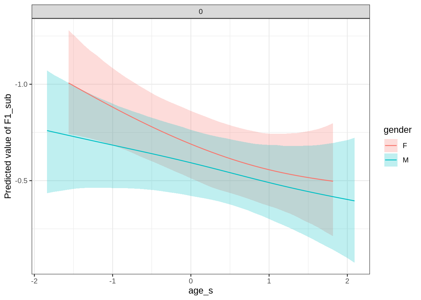
Figure 79 is interestingly different from Figure 20. We see a lower in the vowel space for both female and male preschoolers. Both have means estimated to be outside of the 90% credible interval for the youngest speakers. If anything, this movement in the male preschoolers would make our story easier to tell.
7.2.4 kit F2
We copy the above steps for kit F2.
kit_f2_data <- f2 |>
  filter(
    vowel == "KIT"
  ) |>
  mutate(
    w_s = interaction(word, stressed),
    p_c = interaction(participant, collect)
  ) %>%
  droplevels() |>
  filter(
    !is.na(F2_sub)
)summary(kit_f2_data) participant collect age_s gender word
Length:848 Min. :1.000 Min. :-1.8383 F:471 his :113
Class :character 1st Qu.:2.000 1st Qu.:-0.5942 M:377 him : 88
Mode :character Median :3.000 Median : 0.1523 it : 62
Mean :2.971 Mean : 0.1602 bridge : 43
3rd Qu.:4.000 3rd Qu.: 0.8988 the : 38
Max. :4.000 Max. : 2.1429 baby : 23
(Other):481
vowel stressed stopword F2_sub age
KIT:848 Mode :logical Mode :logical Min. :-7.9086 Min. :47.00
FALSE:286 FALSE:474 1st Qu.:-0.5300 1st Qu.:52.00
TRUE :562 TRUE :374 Median : 0.2657 Median :55.00
Mean : 0.1626 Mean :55.03
3rd Qu.: 0.9259 3rd Qu.:58.00
Max. : 5.2423 Max. :63.00
duration_s w_s p_c
Min. :-0.8373 his.TRUE :105 EC0405-Child.2: 30
1st Qu.:-0.6123 him.TRUE : 84 EC0918-Child.4: 28
Median :-0.2749 it.TRUE : 59 EC0102-Child.4: 23
Mean :-0.1246 bridge.TRUE: 42 EC0901-Child.4: 23
3rd Qu.: 0.1561 the.TRUE : 38 EC0501-Child.1: 21
Max. : 2.4875 baby.FALSE : 23 EC0806-Child.1: 21
(Other) :497 (Other) :702 kit_f2_fit_sub <- brm(
F2_sub ~ gender + stopword +
s(age_s, by=gender, k = 5) +
s(duration_s, k = 5) +
(1 | w_s) +
(1 | p_c),
data = kit_f2_data,
family = student(),
prior = prior_t,
chains = 4,
cores = 4,
iter = 3000,
control = list(adapt_delta = 0.99),
)
write_rds(
kit_f2_fit_sub,
here('models', 'kit_f2_fit_sub.rds'),
compress = "gz"
)kit_f2_preds <- estimate_relation(
kit_f2_fit_sub,
by = list(
age_s = seq(min_age_s, max_age_s, length = 50),
gender = c("F", "M"),
duration_s = 0
),
predict="link",
ci = 0.9
)
kit_f2_preds %>%
plot() +
scale_y_reverse()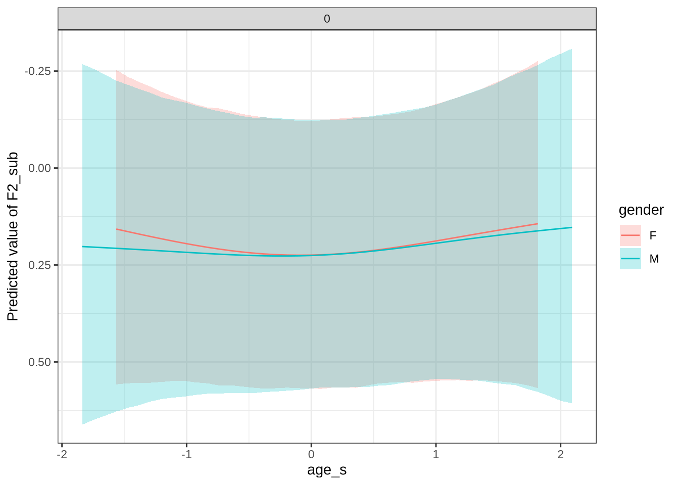
Figure 80 shows now clear evidence of any kind of movement in the vowel space (whereas we expect some backing in the male preschoolers). The credible intervals appear wide, but this is mostly a feature of the scale of the visualization.
References
References
Allaire, JJ, Yihui Xie, Christophe Dervieux, Jonathan McPherson, Javier Luraschi, Kevin Ushey, Aron Atkins, et al. 2024. rmarkdown: Dynamic Documents for r. https://github.com/rstudio/rmarkdown.
Arel-Bundock, Vincent, Noah Greifer, and Andrew Heiss. 2024. ‘How to Interpret Statistical Models Using marginaleffects for R and Python’. Journal of Statistical Software 111 (9): 1–32. https://doi.org/10.18637/jss.v111.i09.
Barreda, Santiago, and Joey Stanley. 2025. fasttrackr: Fast Track Integration in r. https://github.com/santiagobarreda/FastTrackR.
Barthelme, Simon. 2024. imager: Image Processing Library Based on ‘CImg’. https://CRAN.R-project.org/package=imager.
Bořil, Tomáš, and Radek Skarnitzl. 2016. ‘Tools rPraat and mPraat’. In Text, Speech, and Dialogue: 19th International Conference, TSD 2016, Brno, Czech Republic, September 12-16, 2016, Proceedings, edited by Petr Sojka, Aleš Horák, Ivan Kopeček, and Karel Pala, 367–74. Cham: Springer International Publishing. https://doi.org/10.1007/978-3-319-45510-5_42.
Bürkner, Paul-Christian. 2017. ‘brms: An R Package for Bayesian Multilevel Models Using Stan’. Journal of Statistical Software 80 (1): 1–28. https://doi.org/10.18637/jss.v080.i01.
———. 2018. ‘Advanced Bayesian Multilevel Modeling with the R Package brms’. The R Journal 10 (1): 395–411. https://doi.org/10.32614/RJ-2018-017.
———. 2021. ‘Bayesian Item Response Modeling in R with brms and Stan’. Journal of Statistical Software 100 (5): 1–54. https://doi.org/10.18637/jss.v100.i05.
Cameron, Allan, and Teun van den Brand. 2025. geomtextpath: Curved Text in ‘ggplot2’. https://CRAN.R-project.org/package=geomtextpath.
Ching, Travers. 2025. Qs2: Efficient Serialization of r Objects. https://CRAN.R-project.org/package=qs2.
Fromont, Robert. 2025. nzilbb.labbcat: Accessing Data Stored in ‘LaBB-CAT’ Instances. https://CRAN.R-project.org/package=nzilbb.labbcat.
Gabry, Jonah, and Tristan Mahr. 2025. ‘bayesplot: Plotting for Bayesian Models’. https://mc-stan.org/bayesplot/.
Gabry, Jonah, Daniel Simpson, Aki Vehtari, Michael Betancourt, and Andrew Gelman. 2019. ‘Visualization in Bayesian Workflow’. J. R. Stat. Soc. A 182: 389–402. https://doi.org/10.1111/rssa.12378.
Hester, Jim, and Jennifer Bryan. 2024. glue: Interpreted String Literals. https://glue.tidyverse.org/.
Iannone, Richard, and Olivier Roy. 2024. DiagrammeR: Graph/Network Visualization. https://CRAN.R-project.org/package=DiagrammeR.
Kassambara, Alboukadel. 2023. ggcorrplot: Visualization of a Correlation Matrix Using ‘ggplot2’. https://CRAN.R-project.org/package=ggcorrplot.
Kay, Matthew. 2024a. ‘ggdist: Visualizations of Distributions and Uncertainty in the Grammar of Graphics’. IEEE Transactions on Visualization and Computer Graphics 30 (1): 414–24. https://doi.org/10.1109/TVCG.2023.3327195.
———. 2024b. tidybayes: Tidy Data and Geoms for Bayesian Models. https://doi.org/10.5281/zenodo.1308151.
———. 2025. ggdist: Visualizations of Distributions and Uncertainty. https://doi.org/10.5281/zenodo.3879620.
Makowski, Dominique, Mattan S. Ben-Shachar, Brenton M. Wiernik, Indrajeet Patil, Rémi Thériault, and Daniel Lüdecke. 2025. ‘modelbased: An R Package to Make the Most Out of Your Statistical Models Through Marginal Means, Marginal Effects, and Model Predictions.’ Journal of Open Source Software 10 (109): 7969. https://doi.org/10.21105/joss.07969.
Müller, Kirill. 2020. here: A Simpler Way to Find Your Files. https://CRAN.R-project.org/package=here.
Pedersen, Thomas Lin. 2025. ggforce: Accelerating ‘ggplot2’. https://CRAN.R-project.org/package=ggforce.
Pedersen, Thomas Lin, and Fabio Crameri. 2023. scico: Colour Palettes Based on the Scientific Colour-Maps. https://CRAN.R-project.org/package=scico.
R Core Team. 2024. R: A Language and Environment for Statistical Computing. Vienna, Austria: R Foundation for Statistical Computing. https://www.R-project.org/.
Slowikowski, Kamil. 2024. ggrepel: Automatically Position Non-Overlapping Text Labels with ‘ggplot2’. https://CRAN.R-project.org/package=ggrepel.
van Rij, Jacolien, Martijn Wieling, R. Harald Baayen, and Hedderik van Rijn. 2022. ‘itsadug: Interpreting Time Series and Autocorrelated Data Using GAMMs’.
Wickham, Hadley, Mara Averick, Jennifer Bryan, Winston Chang, Lucy D’Agostino McGowan, Romain François, Garrett Grolemund, et al. 2019. ‘Welcome to the tidyverse’. Journal of Open Source Software 4 (43): 1686. https://doi.org/10.21105/joss.01686.
Wilson Black, Joshua, James Brand, Jen Hay, and Lynn Clark. 2023. ‘Using Principal Component Analysis to Explore Co‐variation of Vowels’. Language and Linguistics Compass 17 (1): e12479. https://doi.org/10.1111/lnc3.12479.
Wood, S. N. 2003. ‘Thin-Plate Regression Splines’. Journal of the Royal Statistical Society (B) 65 (1): 95–114. https://doi.org/10.1111/1467-9868.00374.
———. 2004. ‘Stable and Efficient Multiple Smoothing Parameter Estimation for Generalized Additive Models’. Journal of the American Statistical Association 99 (467): 673–86. https://doi.org/10.1198/016214504000000980.
———. 2011. ‘Fast Stable Restricted Maximum Likelihood and Marginal Likelihood Estimation of Semiparametric Generalized Linear Models’. Journal of the Royal Statistical Society (B) 73 (1): 3–36. https://doi.org/10.1111/j.1467-9868.2010.00749.x.
———. 2017. Generalized Additive Models: An Introduction with R. 2nd ed. Chapman; Hall/CRC.
Wood, S. N., N. Pya, and B. Säfken. 2016. ‘Smoothing Parameter and Model Selection for General Smooth Models (with Discussion)’. Journal of the American Statistical Association 111: 1548–75. https://doi.org/10.1080/01621459.2016.1180986.
Xie, Yihui. 2014. ‘knitr: A Comprehensive Tool for Reproducible Research in R’. In Implementing Reproducible Computational Research, edited by Victoria Stodden, Friedrich Leisch, and Roger D. Peng. Chapman; Hall/CRC.
———. 2015. Dynamic Documents with R and Knitr. 2nd ed. Boca Raton, Florida: Chapman; Hall/CRC. https://yihui.org/knitr/.
———. 2024. knitr: A General-Purpose Package for Dynamic Report Generation in r. https://yihui.org/knitr/.
Xie, Yihui, J. J. Allaire, and Garrett Grolemund. 2018. R Markdown: The Definitive Guide. Boca Raton, Florida: Chapman; Hall/CRC. https://bookdown.org/yihui/rmarkdown.
Xie, Yihui, Christophe Dervieux, and Emily Riederer. 2020. R Markdown Cookbook. Boca Raton, Florida: Chapman; Hall/CRC. https://bookdown.org/yihui/rmarkdown-cookbook.
Zhu, Hao. 2024. kableExtra: Construct Complex Table with ‘kable’ and Pipe Syntax. https://CRAN.R-project.org/package=kableExtra.
Footnotes
Code to extract the data from QuakeBox is given in the
scriptsdirectory of the GitHub repository for the project.↩︎
