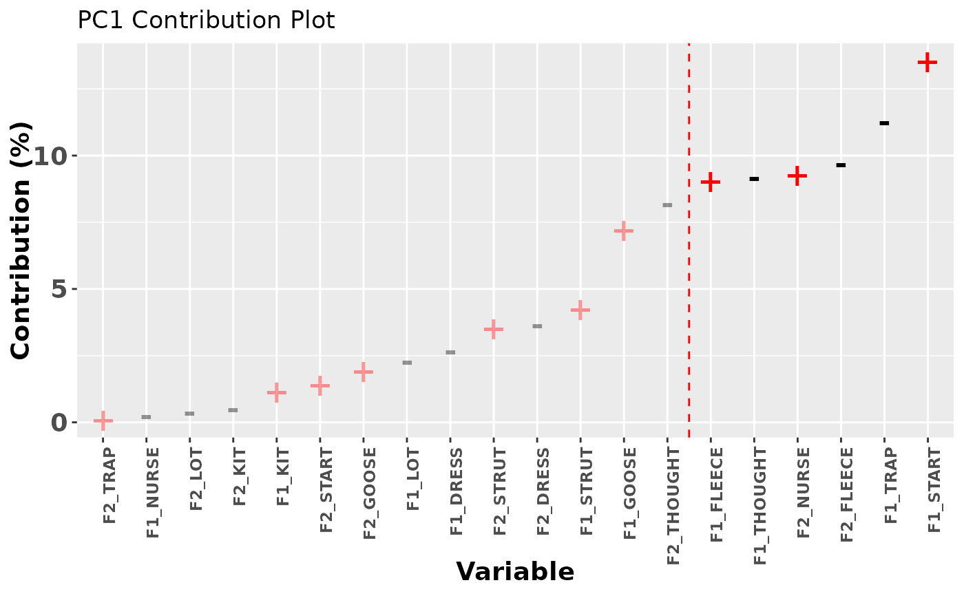
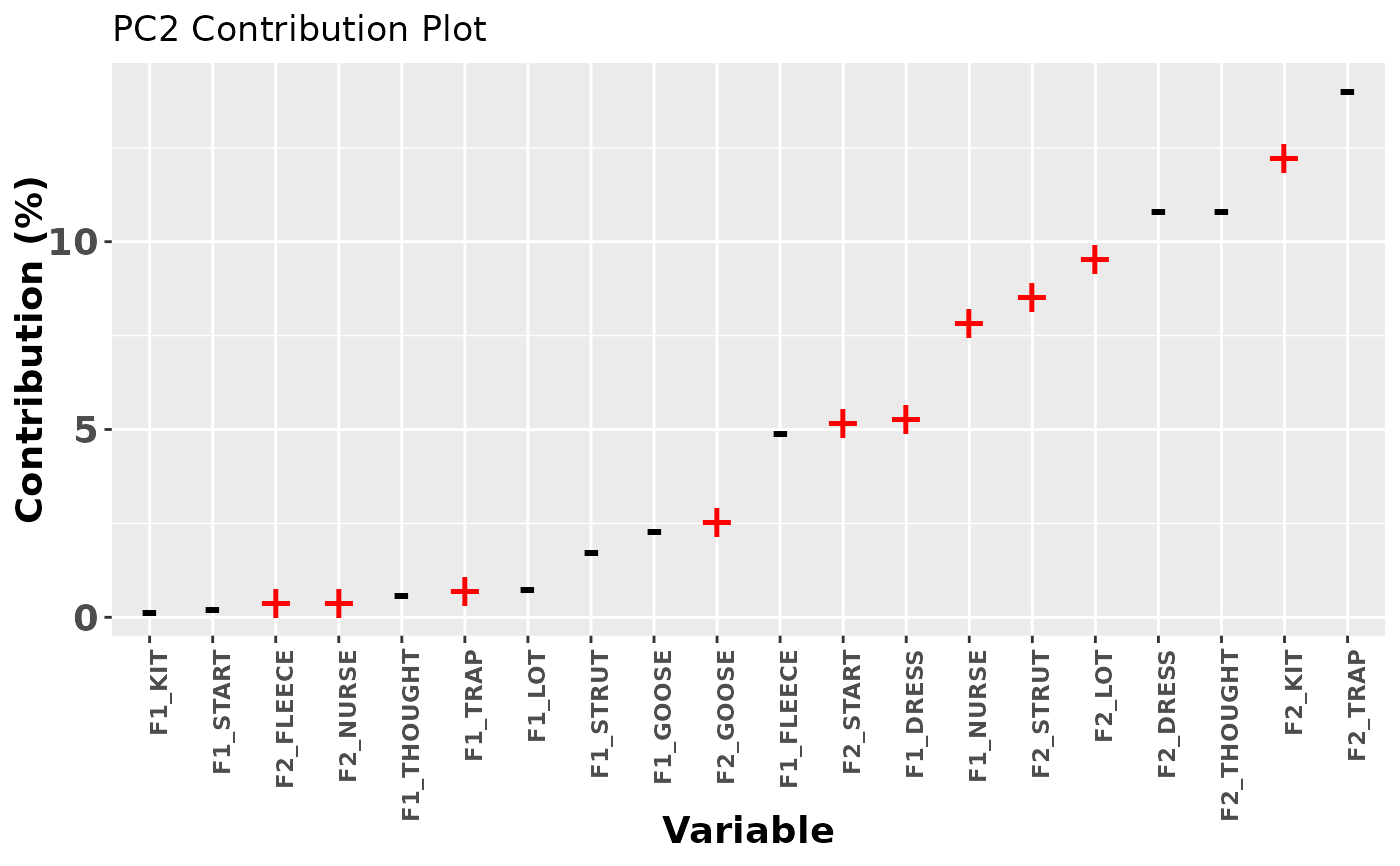
PCA contribution plots — pca_contrib

Plot the contribution of each variable in a data set to a given Principal Component (PC). Variables are arranged by ascending contribution to the PC, where contribution is the squared loading for the variable expressed as a percentage. These plots match those given in supplementary material for Brand et al. (2021).

Usage

pca_contrib_plot(pca_object, pc_no = 1, cutoff = 50)

Arguments

pca_object: a pca object generated by prcomp or princomp.
pc_no: the PC to be visualised. Default value is 1.
cutoff: the cutoff value for interpretation of the PC. Determines what total percentage contribution we want from the variables we select for interpretation. The default of 50 means that we pick the variables with the highest contribution to the PC until we have accounted for 50% of the total contributions to the PC. Can be set to NULL in which case, no cutoff value is plotted.

Value

ggplot object.

Details

As with the other plotting functions in this package, the result is a ggplot2 plot. It can be modified using ggplot2 functions (see, e.g., plot_correlation_magnitudes().

References

Brand, James, Jen Hay, Lynn Clark, Kevin Watson & Márton Sóskuthy (2021): Systematic co-variation of monophthongs across speakers of New Zealand English. Journal of Phonetics. Elsevier. 88. 101096. doi:10.1016/j.wocn.2021.101096

Examples

  onze_pca <- prcomp(onze_intercepts |> dplyr::select(-speaker), scale = TRUE)

  # Plot PC1 with a cutoff value of 60%
  pca_contrib_plot(onze_pca, pc_no = 1, cutoff = 60)


  # Plot PC2 with no cutoff value.
  pca_contrib_plot(onze_pca, pc_no = 2, cutoff = NULL)