1 Why rotate?
It is often useful to apply rotations to the outputs of PCA. This article
demonstrates a few options for rotation using functions from nzilbb.vowels.
First, we discuss the use of rotation for comparing PCA applied across distinct data sets.
We then discuss the use of rotation for PCA applied to a single dataset.
NB: This page should be taken as work-in-progress!
3 Comparing PCA across two data sets
3.1 Are the same patterns of covariation present in two data sets?
Hurring et al. (Under review) show that similar patterns of covariation are present in data from the ONZE corpus and the QuakeBox corpus, two distinct corpora of New Zealand English (NZE).
In order to mimic the results of Hurring et al. (Under review) we apply the model-to-PCA
pipeline to the qb_vowels data included in nzilbb.vowels. This dataset
is a small subset of the data considered by Hurring et al. (Under review) It contains 11
speakers for each of 7 age categories, but is not balanced by gender.
qb_models <- qb_vowels |>
  # normalize
  lobanov_2() |>
  pivot_longer(
    cols = c("F1_lob2", "F2_lob2"),
    names_to = "formant_type",
    values_to = "formant_value"
  ) |>
  # changes for compatibility with GAMM modellings.
  mutate(
    speaker = factor(speaker),
    word = factor(word),
    gender = factor(participant_gender),
    age_numeric = as.numeric(factor(participant_age_category))
  ) |>
  # We'll remove FOOT
  filter(
    vowel != "FOOT"
  ) |>
  group_by(vowel, formant_type) |>
  nest() |>
  mutate(
    model = map(
      data,
      ~ bam(
        formant_value ~ gender +
          s(age_numeric, by=gender, k = 4) +
          s(word_freq, k=4) +
          s(articulation_rate, k=4) +
          s(word, bs="re") +
          s(speaker, bs="re"),
        data = .x,
        discrete = TRUE,
        nthreads = 8
      )
    )
  )
Let’s have a look at the predictions from these models. The code below is borrowed from the model-to-PCA vignette.
to_predict <- list(
  "age_numeric" = seq(from=1, to=7, by=1), # All age categories.
  "gender" = c("M", "F")
)

qb_preds <- qb_models |>
  mutate(
    prediction = map(
      model,
      ~ get_predictions(model = .x, cond = to_predict, print.summary = FALSE)
    )
  ) |>
  select(
    vowel, formant_type, prediction
  ) |>
  unnest(prediction) |>
  arrange(
    desc(age_numeric)
  ) |>
  pivot_wider( # Pivot
    names_from = formant_type,
    values_from = c(fit, CI)
  ) |>
  rename(
    F1_lob2 = fit_F1_lob2,
    F2_lob2 = fit_F2_lob2
  )

vowel_colours <- c(
  DRESS = "#777777", # This is the 'bad data' colour for maps
  FLEECE = "#882E72",
  GOOSE = "#4EB265",
  KIT = "#7BAFDE",
  LOT = "#DC050C",
  TRAP = "#878100", # "#F7F056",
  START = "#1965B0",
  STRUT = "#F4A736",
  THOUGHT = "#72190E",
  NURSE = "#E8601C",
  FOOT = "#5289C7"
)

# add labels to data for plotting purposes
qb_preds <- qb_preds |>
    group_by(vowel, gender) |>
    mutate(
      vowel_lab = if_else(
        age_numeric == max(age_numeric),
        vowel,
        ""
      )
    ) |>
    ungroup()

qb_preds |>
  ggplot(
    aes(
      x = F2_lob2,
      y = F1_lob2,
      colour = vowel,
      label = vowel_lab,
      group = vowel
    )
  ) +
  geom_path(
    arrow = arrow(
        ends = "last",
        type="closed",
        length = unit(2, "mm")
      ),
    linewidth = 1
  ) +
  geom_point(
    data = ~ .x |>
      filter(
        !vowel_lab == ""
      ),
    show.legend = FALSE,
    size = 1.5
  ) +
  geom_label_repel(
    min.segment.length = 0, seed = 42,
    show.legend = FALSE,
    fontface = "bold",
    size = 10 / .pt,
    label.padding = unit(0.2, "lines"),
    alpha = 1,
    max.overlaps = Inf
  ) +
  scale_x_reverse(expand = expansion(mult = 0.2), position = "top") +
  scale_y_reverse(expand = expansion(mult = 0.1), position = "right") +
  scale_colour_manual(values = vowel_colours) +
  facet_grid(
      cols = vars(gender)
  ) +
  labs(
    x = "F2 (normalised)",
    y = "F1 (normalised)"
  ) +
  theme(
    plot.title = element_text(face="bold"),
    legend.position="none"
  )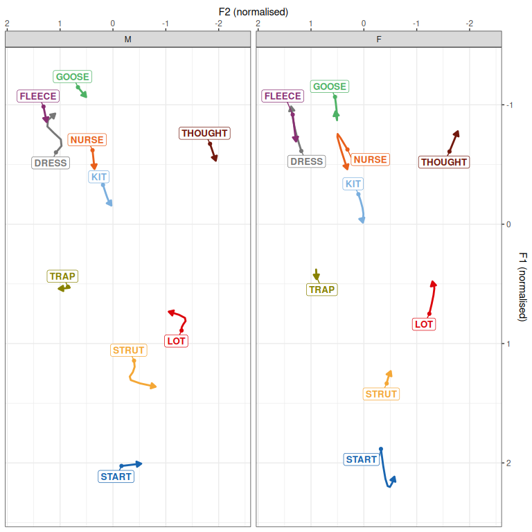
Figure 3.1: Predictions from QuakeBox models.
The trajectories in Figure 3.1 are in line with those found in Hurring et al. (Under review). As we’re interested in PCA rotation here, we’ll skip model criticism and go straight to extracting random intercepts.
qb_intercepts <- qb_models |>
  mutate(
    random_intercepts = map(
      model,
      ~ get_random(.x)$`s(speaker)` |>
        as_tibble(rownames = "speaker") |>
        rename(intercept = value)
    )
  ) |>
  select(
    vowel, formant_type, random_intercepts
  ) |>
  unnest(random_intercepts) |>
  arrange(as.character(vowel)) |>
  ungroup() |>
  mutate(
    # Combine the 'vowel' and 'formant_type' columns as a string.
    vowel_formant = str_c(vowel, '_', formant_type),
    # Remove '_lob2' for cleaner column names
    vowel_formant = str_replace(vowel_formant, '_lob2', '')
  ) |>
  ungroup() |>
  # Remove old 'vowel' and 'formant_type' columns
  select(-c(vowel, formant_type)) |>
  # Make data 'wider', by...
  pivot_wider(
    names_from = vowel_formant, # naming columns using 'vowel_formant'...
    values_from = intercept # and values from intercept column
  ) %>%
  # take only complete cases (some speakers don't have enough vowels for models)
  # NB: a use for the magrittr pipe rather than the native R pipe.
  filter(
    complete.cases(.)
  )
Now let’s do some PCA with these new intercepts and with the onze intercepts from Brand et al. (2021).
qb_pca_test <- pca_test(
  qb_intercepts |> select(-speaker),
  n = 100
)

# change variable names to match QB. QB names are of form VOWEL_FORMANT. ONZE
# names are of formant FORMANT_VOWEL.
onze_intercepts_full <- onze_intercepts_full |>
  rename_with(
    ~ paste0(
      str_extract(.x, "_([A-Z]*)", group=1),
      "_",
      str_extract(.x, "F[1-2]")
    ),
    .cols = matches("F[0-9]")
  )

onze_pca_test <- pca_test(
  onze_intercepts_full |> select(-speaker),
  n = 100
)
We’ll look at the variances explained by each.
plot_variance_explained(qb_pca_test)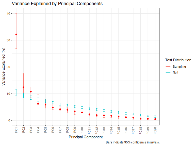
Figure 3.2: Variance explained by QB PCs.
plot_variance_explained(onze_pca_test)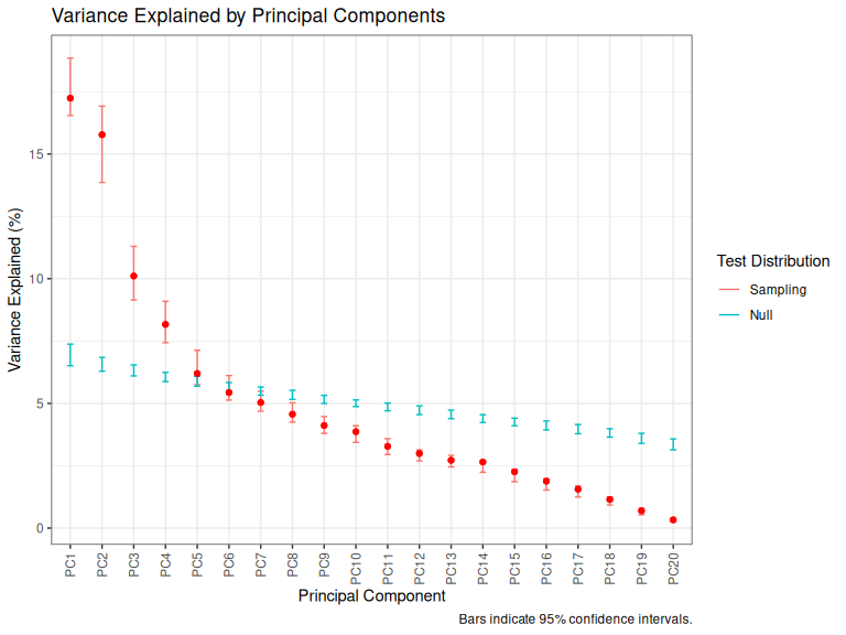
Figure 3.3: Variance explained by ONZE PCs.
Let’s look at the first two PCs of each to see if there’s any similarity in the patterns which emerge.
loadings_to_plot <- bind_rows(
  "QB" = qb_pca_test$loadings,
  "ONZE" = onze_pca_test$loadings,
  .id = "Corpus"
)

loadings_to_plot |>
  pivot_wider(
    names_from = "PC",
    values_from = low_null:sig_loading
  ) |>
  # annoyingly the variables are of form Fx_VOWEL in ONZE and VOWEL_Fx in QB.
  # we change to match QB
  ggplot(
    aes(
      xend = loading_PC1,
      yend = loading_PC2,
      label = variable
    )
  ) +
  geom_segment(x=0, y=0, arrow = arrow(length = unit(2, "mm"))) +
  geom_label_repel(aes(x=loading_PC1, y = loading_PC2), size = 2) +
  scale_x_continuous(expand = expansion(mult=0.1)) +
  facet_grid(cols = vars(Corpus))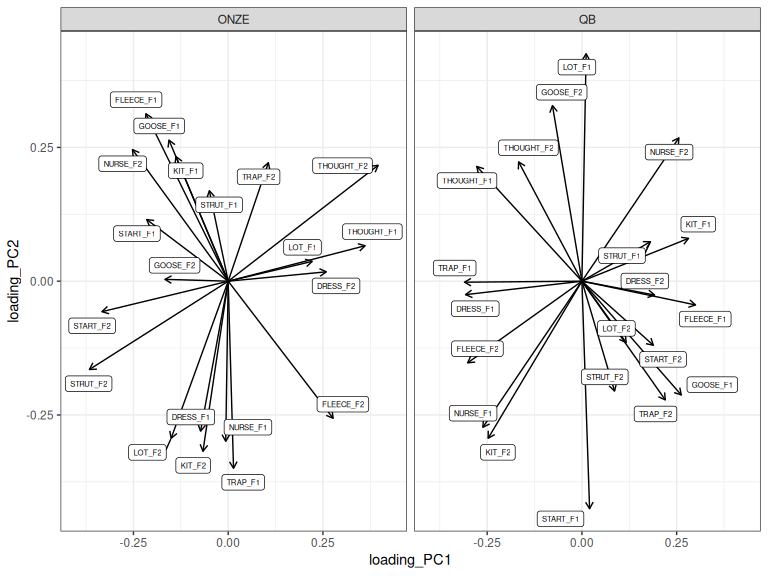
Figure 3.4: Loadings for PC1 and PC2 across ONZE and QB.
Spend some time peering at Figure 3.4. You will start to see patterns which are common to both, but which are not captured by just looking at PC1 or PC2.
Hurring et al. (Under review) focuses on similarity between the two corpora and finds this by means of looking at loadings by themselves. They find a nice correspondence between PC2 in ONZE and PC1 in QB.1 It was nice for their argument that nothing special was done to the PCs which might suggest rigging things in favour of finding similarities.
If, instead, we’re interested in meaningful differences between patterns in the two corpora. We might want to maximise the similarity between the two before interpreting differences. This can be achieved by rotation.
At this point it is worth emphasising the variance of PCA in the sense of large changes in PC loadings with small changes in the input data. Variance in loadings is particularly high in cases where there are multiple PCs which explain similar amounts of variance to one another. This is the point of the confidence intervals around the plots of variance explained above. If, as in Figure 3.3, PC1 and PC2 have overlapping confidence intervals, then we expect that there will be a lot of variance in which variables get loaded on which PC (or on some combination of both PCs).
This kind of instability can be very easily visualised by showing PC1 and PC2 for the ONZE data across 15 bootstrapped samples.
set.seed(7)

data_boots <- bootstraps(onze_intercepts_full |> select(-speaker), times = 15)

onze_bootstrapped <- tibble(
  iteration = 1:15,
  pca = map(
    data_boots$splits,
    ~ prcomp(
      as_tibble(.x),
      scale = TRUE
    )
  )
)

onze_bootstrapped <- onze_bootstrapped |>
  mutate(
    PC1_loadings = map(
      pca, ~ .x$rotation[, 1]
    ),
    PC2_loadings = map(
      pca, ~ .x$rotation[, 2]
    ),
    variable = map(
      pca, ~ rownames(.x$rotation)
    )
  )

onze_loadings <- onze_bootstrapped |>
  # ditch 'scores' columns
  select(
    -contains('_scores'), -pca
  ) |>
  unnest(c(PC1_loadings, PC2_loadings, variable)) |>
  rename(
    PC1 = PC1_loadings,
    PC2 = PC2_loadings
  ) |>
  mutate(
    pattern = case_when(
      variable %in% c("THOUGHT_F2", "STRUT_F2", "THOUGHT_F1", "START_F2") ~
        "Back vowel configuration",
      variable %in% c(
        "TRAP_F1", "KIT_F2", "FLEECE_F1", "NURSE_F1", "LOT_F2", "DRESS_F1"
      ) ~ "Leader/lagger",
      .default = "Other"
    )
  )

anim <- onze_loadings |>
  ggplot(
    aes(
      x = PC1,
      y = PC2,
      xend = PC1,
      yend = PC2,
      label = variable,
      group = variable,
      colour = pattern
    )
  ) +
  geom_hline(
    yintercept = 0,
    linewidth = 0.5,
    linetype = "dashed"
  ) +
  geom_vline(
    xintercept = 0,
    linewidth = 0.5,
    linetype = "dashed"
  ) +
  geom_segment(
    x = 0,
    y = 0,
    arrow = arrow(),
    #show.legend = FALSE,
    linewidth = 1.5
  ) +
  geom_text(
    size = 5,
    show.legend = FALSE,
    nudge_x = 0.05,
    nudge_y = 0.05
  ) +
  scale_colour_manual(
    values = c(
      "Leader/lagger" = "#F95A5C",
      "Back vowel configuration" = "#425B78",
      "Other" = "grey"
    )
  ) +
  scale_x_continuous(expand = expansion(mult=0.1)) +
  scale_y_continuous(expand = expansion(mult=0.1)) +
  theme_minimal() +
  theme(
    plot.caption = element_text(size = 20),
  ) +
  labs(
    caption = "Bootstrap: {closest_state}/15",
    colour = "Vowel pattern"
  ) +
  transition_states(
    iteration,
    transition_length = 4,
    state_length = 2
  )

animate(anim, nframes = 500)
Figure 3.5: Variation in PC1 and PC2 loadings (ONZE).
The moral of Figure 3.5 is that the same patterns are pretty consistent even if they switch between PC1 and PC2 or their polarity switches from negative to positive. The red collection of arrows and the blue collections of arrows show the ‘leader/lagger’ and the ‘back vowel configuration’ patterns identified by Brand et al. These relative positions of the arrows in these patterns is consistent, but they are captured differently in PC1 and PC2 space in different samples from the original data.
When it comes to comparing ONZE with QB, we are not interested if a pattern is captured by PC1 in one corpus and PC2 in the other. This might indicate something about the relative strength of the patterns in the community, but only if the confidence intervals for variance explained by PC1 and PC2 did not overlap for both corpora (i.e., both Figure 3.3 and Figure 3.2 show PCs which do not have overlapping confidence intervals).
3.1.1 Manual rotation
Sometimes, if we are working with two PCs, it’s easiest to just decide how much
we want to rotate a space and manually do it. nzilbb.vowels includes the
pca_rotate_2d() to rotate PCs in two dimensions. It works for the output
of prcomp() and princomp(), but not for the output of pca_test().
Let’s repeat Figure 3.4 with prcomp().
qb_pca <- prcomp(
  qb_intercepts |> select(-speaker),
  scale = TRUE
)

onze_pca <- prcomp(
  onze_intercepts_full |> select(-speaker),
  scale = TRUE
)

loadings_to_plot <- bind_rows(
  "QB" = as_tibble(qb_pca$rotation, rownames="variable"),
  "ONZE" = as_tibble(onze_pca$rotation, rownames="variable"),
  .id = "Corpus"
)

loadings_to_plot |>
  ggplot(
    aes(
      xend = PC1,
      yend = PC2,
      label = variable
    )
  ) +
  geom_segment(x=0, y=0, arrow = arrow(length = unit(2, "mm"))) +
  geom_label_repel(aes(x=PC1, y = PC2), size = 2) +
  scale_x_continuous(expand = expansion(mult=0.1)) +
  facet_grid(cols = vars(Corpus))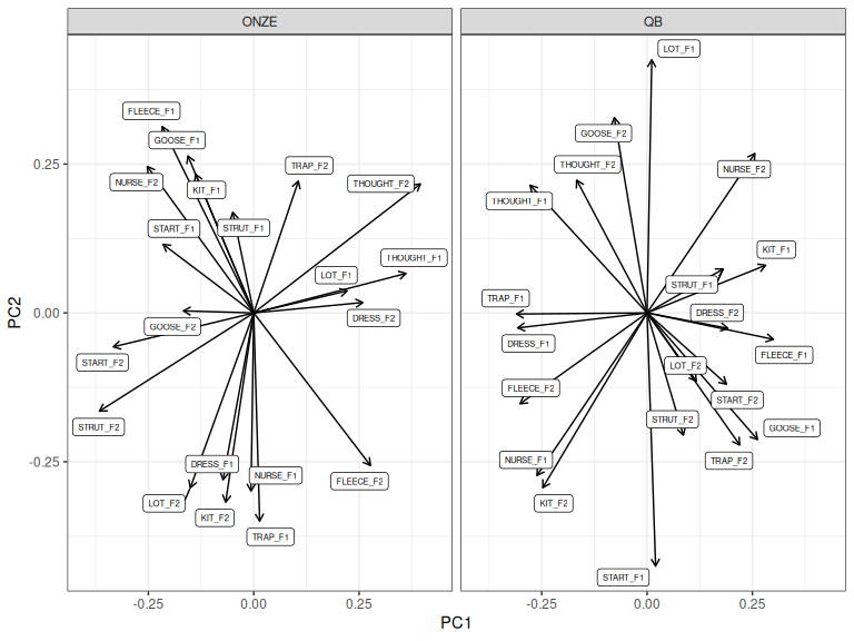
Figure 3.6: ONZE and QB loadings for PC1 and PC2 before rotation.
Let’s align ONZE with QB. Visually, we can see that this is possible by rotating
TRAP_F1 in both along PC1. A roughly 90 degree clockwise rotation would
achieve this. Let’s do it.
onze_rot <- pca_rotate_2d(onze_pca, 90, pcs=c(1,2))

loadings_to_plot <- bind_rows(
  "QB" = as_tibble(qb_pca$rotation, rownames="variable"),
  "ONZE (Rotated)" = as_tibble(onze_rot$rotation, rownames="variable"),
  .id = "Corpus"
)

loadings_to_plot |>
  ggplot(
    aes(
      xend = PC1,
      yend = PC2,
      label = variable
    )
  ) +
  geom_segment(x=0, y=0, arrow = arrow(length = unit(2, "mm"))) +
  geom_label_repel(aes(x=PC1, y = PC2), size = 2) +
  scale_x_continuous(expand = expansion(mult=0.1)) +
  facet_grid(cols = vars(Corpus)) +
  labs(
    x = "Component 1",
    y = "Component 2"
  )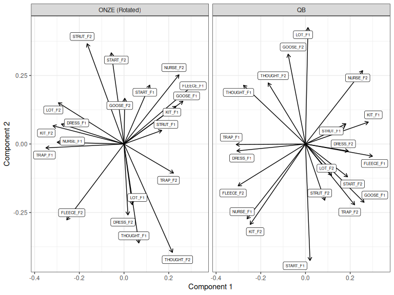
Figure 3.7: ONZE and QB loadings for components 1 and 2, ONZE rotated.
Figure 3.7 roughly aligns the first component in ONZE with the first
PC in QB.2
It looks like the second component would be more similar if we also flip the
ONZE second component. Let’s do this using the pc_flip() function.
onze_rot <- pc_flip(onze_rot, pc_no=2)

loadings_to_plot <- bind_rows(
  "QB" = as_tibble(qb_pca$rotation, rownames="variable"),
  "ONZE (Rotated and flipped)" = as_tibble(onze_rot$rotation, rownames="variable"),
  .id = "Corpus"
)

loadings_to_plot |>
  ggplot(
    aes(
      xend = PC1,
      yend = PC2,
      label = variable
    )
  ) +
  geom_segment(x=0, y=0, arrow = arrow(length = unit(2, "mm"))) +
  geom_label_repel(aes(x=PC1, y = PC2), size = 2) +
  scale_x_continuous(expand = expansion(mult=0.1)) +
  facet_grid(cols = vars(Corpus)) +
  labs(
    x = "Component 1",
    y = "Component 2"
  )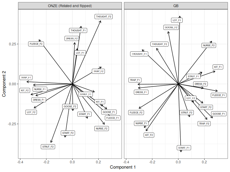
Figure 3.8: ONZE and QB loadings for components 1 and 2, ONZE manually rotated and then flipped on Component 2.
It is only arguable that this flip improves things. We could test this using correlations, but it would better to switch to a less impressionistic method. Nonetheless, simple 2D rotations and flips, manually applied, are sometimes all that you need.
3.1.2 Procrustes rotation
Procrustes rotation produces the closest alignment between two shapes which is possible using scaling and rotation. The two shapes must have the same landmarks as each other. In our case, the shape is the position of each of our variables in the space defined by the PCs, that is, the loadings.3
Underlying this method is the procrustes() function from the vegan package.
As with the other uses of PCA in the NZILBB research programme that
nzilbb.vowels has emerged from, we are close to ‘ordination’ methods used in
community ecology. vegan is a package from community ecology. For
nzilbb.vowels, I have hidden the options which explicitly use the language of
‘species’ and ‘site’. The nzilbb.vowels function is called
pca_rotate_procrustes().
We will now maximally align the QB and ONZE PCA analyses using Procrustes
rotation. We have to choose how many PCs to include when we do this. For the
purposes of this illustration, we will choose the first five PCs, because the
ONZE data has five statistically significant PCs according to pca_test().4 We will again rotate ONZE to match QB (but we could
easily go the other way).
NB: We have to ensure that the order in which the variables appear in the
data which goes into prcomp() is the same across the two PCAs. This is how
the Procrustes function aligns the variables in the two datasets. For instance,
if the first dataset has columns in order “DRESS_F1”, “KIT_F1”, “DRESS_F2”,
and the seecond has columns in order “DRESS_F1”, “DRESS_F2”, “KIT_F1”, then
the Procrustes function will try to align
kit F1 in the first data set
with dress F2 in the second. This
is not what you want!
onze_proc <- onze_pca |>
  pca_rotate_procrustes(target = qb_pca, max_pcs = 5)

loadings_to_plot <- bind_rows(
  "QB" = as_tibble(qb_pca$rotation, rownames="variable"),
  "ONZE (Rotated)" = as_tibble(onze_proc$rotation, rownames="variable"),
  .id = "Corpus"
)

loadings_to_plot |>
  ggplot(
    aes(
      xend = PC1,
      yend = PC2,
      label = variable
    )
  ) +
  geom_segment(x=0, y=0, arrow = arrow(length = unit(2, "mm"))) +
  geom_label_repel(aes(x=PC1, y = PC2), size = 2) +
  scale_x_continuous(expand = expansion(mult=0.1)) +
  facet_grid(cols = vars(Corpus)) +
  labs(
    x = "Component 1",
    y = "Component 2"
  )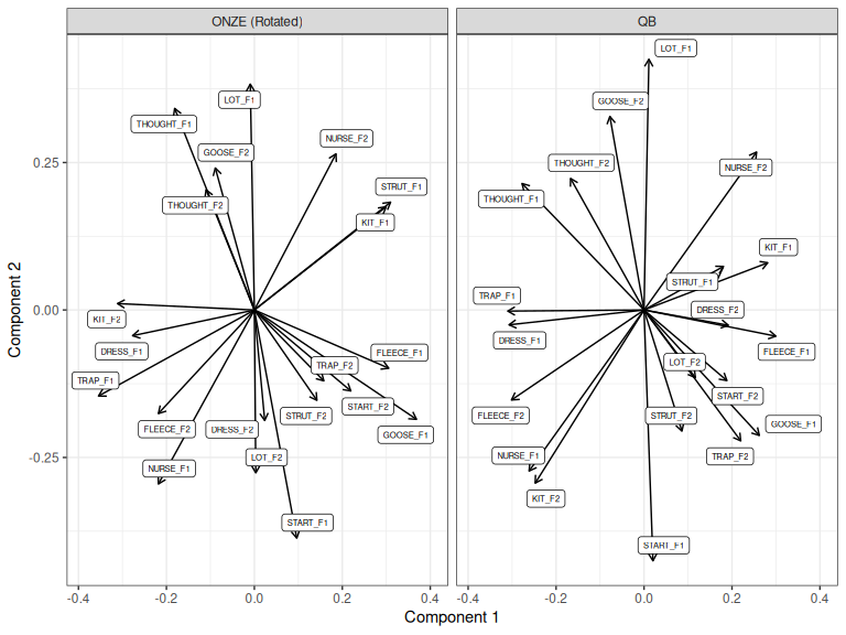
Figure 3.9: First two components of QB PCA and Procrustes rotated ONZE PCA.
How does this compare to the manual rotation we tried above (Figure 3.8)?
loadings_to_plot <- bind_rows(
  "ONZE manual" = as_tibble(onze_rot$rotation, rownames="variable"),
  "ONZE Procrustes" = as_tibble(onze_proc$rotation, rownames="variable"),
  .id = "Corpus"
)

loadings_to_plot |>
  ggplot(
    aes(
      xend = PC1,
      yend = PC2,
      label = variable
    )
  ) +
  geom_segment(x=0, y=0, arrow = arrow(length = unit(2, "mm"))) +
  geom_label_repel(aes(x=PC1, y = PC2), size = 2) +
  scale_x_continuous(expand = expansion(mult=0.1)) +
  facet_grid(cols = vars(Corpus)) +
  labs(
    x = "Component 1",
    y = "Component 2"
  )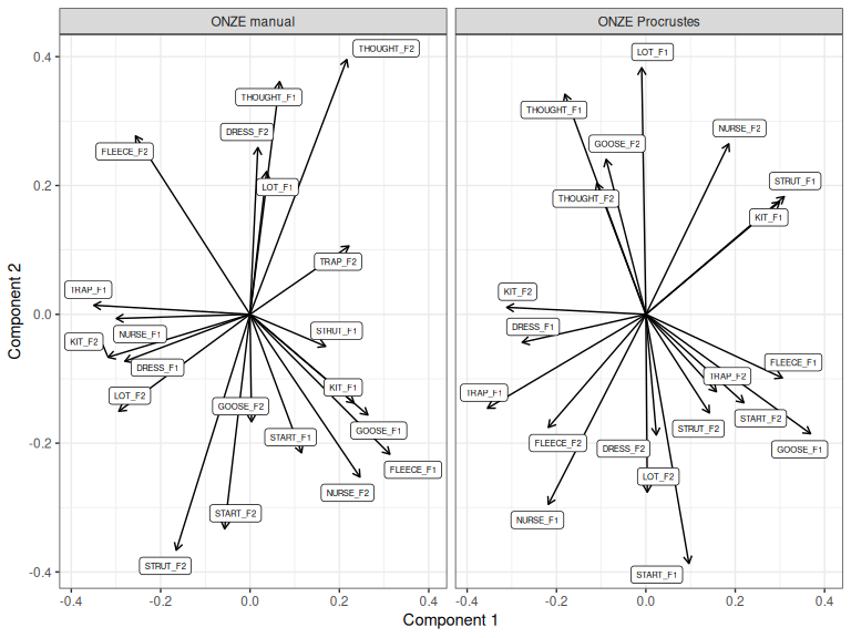
Figure 3.10: ONZE PCA rotated manually and via Procrustes rotation.
The biggest difference between the two approaches is that this Procrustes rotation is a five dimensional rotation, whereas the manual rotation is only 2D. Information from any of the first 5 dimensions picked up by Procrustes rotation can now appear in Component 1 or Component 2, with the aim of matching the patterns present in the first five PCs of the QuakeBox.
The manual rotation, in this case, does more closely match the interpretation where Component 1 measures something like ‘leader/lagger’ status and the second component gives us some kind of change in back vowel configuration. This is unsurprising, as that interpretation is what motivated the selection of the manual rotation which we applied!
3.2 Partial overlap of variables and rotation on scores
In some cases, we might have partially overlapping variables in our two PCA analyses. Upcoming work on bilingualism faces this problem, where only some vowel categories can be aligned across languages.
There is no special issue for manual 2D rotations. The problem is slightly more serious for Procrustes rotation. The solution is to work out the rotation using the shared landmarks and then apply the rotation to all variables.
We can specify which landmarks to use via the rotation_variables
argument to pca_rotate_procrustes(). We list the names of each variable
we will use in a vector. This implies that the names of the variables are the
same in each dataset. We’ll rotate using just DRESS, TRAP, and KIT.
rot_vars <- c(
  "DRESS_F1", "DRESS_F2", "TRAP_F1", "TRAP_F2", "KIT_F1", "KIT_F2"
)

onze_proc <- onze_pca |>
  pca_rotate_procrustes(
    target = qb_pca,
    max_pcs = 3, # Exercise: look at what happens when you change this.
    rotation_variables = rot_vars
  )

loadings_to_plot <- bind_rows(
  "QB" = as_tibble(qb_pca$rotation, rownames="variable"),
  "ONZE (Rotated)" = as_tibble(onze_proc$rotation, rownames="variable"),
  .id = "Corpus"
)

loadings_to_plot |>
  mutate(
    highlight = str_detect(variable, "(DRESS|TRAP|KIT)")
  ) |>
  ggplot(
    aes(
      xend = PC1,
      yend = PC2,
      label = variable,
      fill = highlight,
      colour = highlight
    )
  ) +
  geom_segment(x=0, y=0, arrow = arrow(length = unit(2, "mm"))) +
  geom_label_repel(aes(x=PC1, y = PC2), size = 2, colour="black") +
  scale_x_continuous(expand = expansion(mult=0.1)) +
  scale_fill_manual(
    values = c("TRUE" = "red", "FALSE" = "grey")
  ) +
  scale_colour_manual(
    values = c("TRUE" = "red", "FALSE" = "grey")
  ) +
  facet_grid(cols = vars(Corpus)) +
  labs(
    x = "Component 1",
    y = "Component 2"
  ) +
  theme(
    legend.position = "none"
  )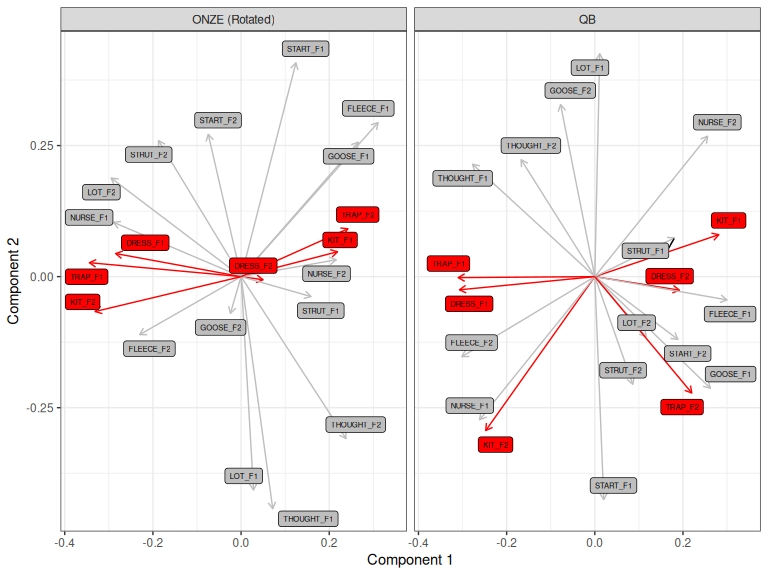
Figure 3.11: QB1 PCA and Procrustes rotated ONZE PCA, rotated with respect to DRESS, TRAP, and KIT only.
If you are in the lucky position that you have the exact same speakers in both corpora, then you can rotate by scores instead and then determine what happens to the variables. The individuals must be in the same order in both datasets. This is not the case for the QuakeBox and ONZE corpora, but it is the case for a subset of the QuakeBox corpora.
QB1_ints <- read_rds('data/QB1_scores_anon.rds') |>
  select(-contains("PC"))
QB2_ints <- read_rds('data/QB2_scores_anon.rds')|>
  select(-contains("PC"))
Let’s apply procrustes rotation to the scores and then look at what this does to the interpretation of the loadings.
# get shared speakers between QB1 and QB2 and ensure they are in the same
# order in the data.
shared_speakers = intersect(QB1_ints$speaker, QB2_ints$speaker)

QB1_ints <- QB1_ints |>
  filter(
    speaker %in% shared_speakers
  ) |>
  arrange(speaker)

QB2_ints <- QB2_ints |>
  filter(
    speaker %in% shared_speakers
  ) |>
  arrange(speaker)

QB1_pca <- prcomp(
  QB1_ints |> select(-speaker), scale = TRUE
)

QB2_pca <- prcomp(
  QB2_ints |> select(-speaker), scale = TRUE
)
We apply the rotation to QB2, using the scores from each.
# Here it would be a good idea to determine how many PCs to include via
# `pca_test()`. We skip this detail for now.
QB2_proc <- QB2_pca |>
  pca_rotate_procrustes(
    target = QB1_pca,
    max_pcs = 2,
    rotate = "scores"
  )
What does this do to the variance explained by QB2 PCA?
plot(QB2_proc)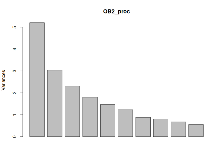
Figure 3.12: Variance explained by components after Procrustes rotation.
Let’s look at the loadings.
loadings_to_plot <- bind_rows(
  "QB1" = as_tibble(QB1_pca$rotation, rownames="variable"),
  "QB2 (Rotated)" = as_tibble(QB2_proc$rotation, rownames="variable"),
  .id = "Corpus"
)

loadings_to_plot |>
  ggplot(
    aes(
      xend = PC1,
      yend = PC2,
      label = variable
    )
  ) +
  geom_segment(x=0, y=0, arrow = arrow(length = unit(2, "mm"))) +
  geom_label_repel(aes(x=PC1, y = PC2), size = 2) +
  scale_x_continuous(expand = expansion(mult=0.1)) +
  facet_grid(cols = vars(Corpus)) +
  labs(
    x = "Component 1",
    y = "Component 2"
  )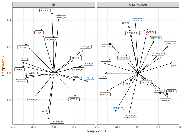
Figure 3.13: Loadings for first two compnents for QB1 PCA and rotated QB2 PCA.
These look very similar to one another. What they say is that if we maximally align the speakers across the two datasets in a space of variation, the linguistic interpretation of this variation stays similar.
To repeat: we have here used Procrustes rotation to rotate the scores for speakers rather than the loadings for variables. We have then looked at the loadings.
But how much variation is there in the scores after rotation?
scores_to_plot <- bind_rows(
  "QB1" = as_tibble(QB1_pca$x, rownames="speaker"),
  "QB2 (Rotated)" = as_tibble(QB2_proc$x, rownames="speaker"),
  .id = "Corpus"
)

scores_to_plot |>
  ggplot(
    aes(
      x = PC1,
      y = PC2,
      group = speaker
    )
  ) +
  geom_vline(xintercept = 0, linewidth = 0.5, linetype = "dashed") +
  geom_hline(yintercept = 0, linewidth = 0.5, linetype = "dashed") +
  geom_line(arrow = arrow(length = unit(2, "mm"))) +
  scale_x_continuous(expand = expansion(mult=0.1)) +
  labs(
    x = "Component 1",
    y = "Component 2"
  )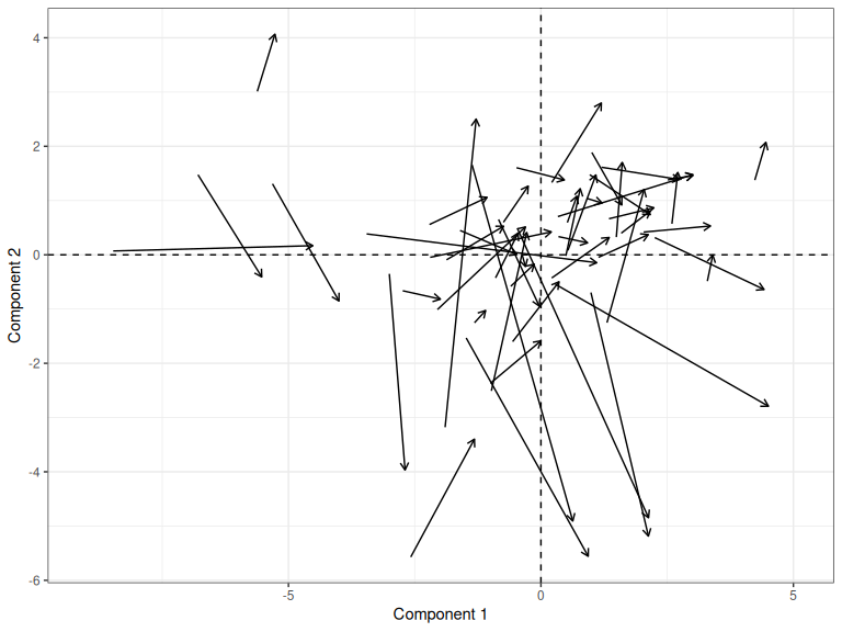
Figure 3.14: Change in PC scores from QB1 to QB2, after Procrustes rotation.
This approach would work even if the two datasets had no variables in common.
4 Rotation for single data set
4.1 Manual rotation for interpretability
Sometimes the interpretability of a space generated by PCA would be much easier if we apply a rotation.
This kind of move is justified if we are more interested in the space captured by the first \(n\) PCs rather than the PCs themselves (Jolliffe 2002, 270).
In this kind of case, justify the number of PCs you consider using
plot_variance_explained() as usual, then apply a manual rotation after looking
at a variable plot. A worked example will be added here in the near future.
4.2 Procrustes rotation for improved confidence bars
We can use Procrustes rotation as an alternative source of confidence bars for loadings. This is currently being explored as an alternative to filtering the bootstraps so that we get cases where the PCs are more-or-less aligned.
This use of Procrustes rotation as part of bootstrapping is common in Multidimensional Scaling (MDS).
The fundamental idea is the same as for the case of comparing across two datasets, for each bootstrap sample is a distinct dataset (explored above).
We implement the test in procrustes_loadings() and plot these with
plot_procrustes_loadings(). If we decide that this is the better way to go for
generating confidence bands, it will be eventually merged into the pca_test()
function.5
The procrustes_loadings() function takes the data you would usually put in
to prcomp() or princomp(). You have to choose a number of PCs to rotate
(the max_pcs argument). One way to make this choice is to use the output of
pca_test() (specifically, the number of ‘statistically significant’ PCs,
as determined by looking at the plot of variance explained). We choose 5
PCs, in line with Figure 3.3.
Let’s generate a distribution of signed index loadings for the first 5
PCs, using the procrustes_loadings() function on the ONZE data.
onze_loadings <- procrustes_loadings(
  onze_intercepts_full |> select(-speaker),
  max_pcs = 5,
  index = TRUE,
  n = 500,
  scale = TRUE
)
The procrustes_loadings() function gives you signed index loadings for each PC
for the bootstrapped analyses (with value Sampling in the source column).
The plot_procrustes_loadings() function can then be used to visualise the
distribution.
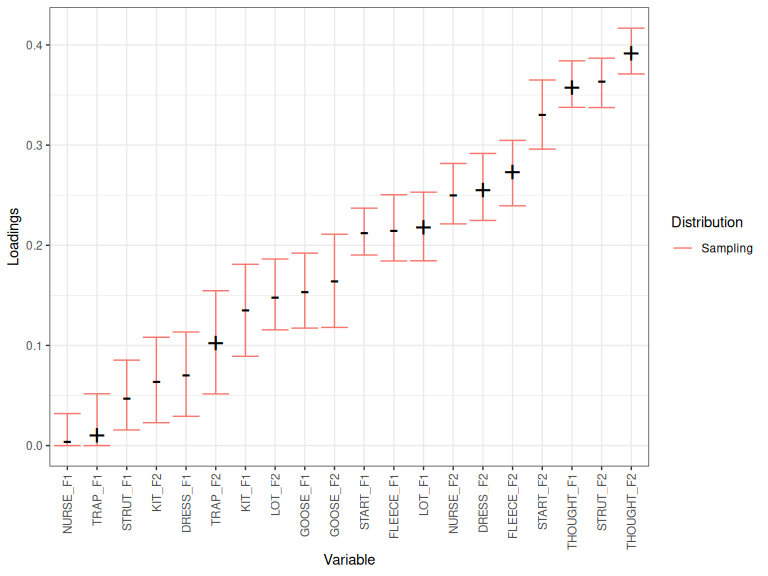
plot_procrustes_loadings(onze_loadings, pc_no=1, loadings_confint = 0.95)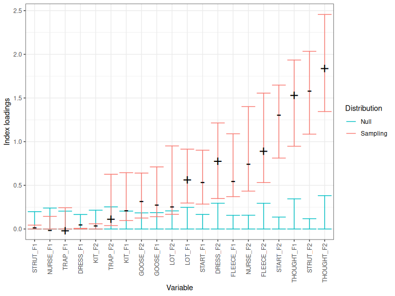
Figure 4.1: Index loadings, confidence band, and null distribution for PC1.
By default, the function uses index loadings (as does pca_test()). But
index loadings are always positive. For the rotation to make sense, we need to
add the sign back to the index loadings (i.e., whether the original loading
is positive or negative). You can generate confidence intervals for the
original loadings by setting index=FALSE.
However, if you set index=FALSE, you will not get an estimate of the null
distribution, and so you won’t get any kind of indication of whether the
loading is itself significant. For instance:
onze_loadings <- procrustes_loadings(
  onze_intercepts_full |> select(-speaker),
  max_pcs = 5,
  index = FALSE,
  n = 500,
  scale = TRUE
)

plot_procrustes_loadings(onze_loadings, pc_no=1, loadings_confint = 0.95)