# We load three packages from the 'tidyverse' by name. `dplyr` includes
# functions for manipulating data. `readr` includes a series of functions for
# reading data in to R, and `tidyr` to pivot data.
library(dplyr)
library(readr)
library(tidyr)
# This package helps to manage the paths to files.
library(here)2 Data Processing
NoteAccess related workshop materials and data
If you have followed the induction instructions on the homepage, you can access a workshop which is closely related to this chapter, and get access to the data, by entering the following code in the console pane:
usethis::create_from_github(
  "https://github.com/nzilbb/ws-data-processing"
)
In this chapter, we’ll look at some common things you will need to do with data. We will also begin to work with a series of packages called the tidyverse, which implement a series of data processing and visualising techniques on top of base R.
I tend to use the tidyverse when I work with data, but there are many people who prefer “base R” (i.e., not the tidyverse). We will look at some base R approaches as these workshops progress, and especially in this chapter, but the majority of the code I put in front of you will use at least some tidyverse methods.
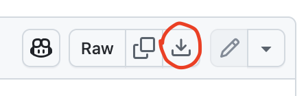
The easiest way to interact with this chapter is to run the code in the callout block above. This will set up a new RStudio project and provide all the data you need. However, you may wish to set up your own project and avoid GitHub. If so, you need to have this data file inside a folder called data inside your project. To download the file after following the link, click the download button at the right of the toolbar.
 Now either make your own new script and enter in the code from each of the blocks below, or open
 scripts/data_processing.R to follow along.
2.1 Processing Data in Base R.
2.1.1 Loading in Data
Usually, you will load data from an external file. It is best practice to treat this file as ‘read only’ for the purposes of your R project. That is, you shouldn’t be overwriting the data file in the course of your project.
Usually this data will be either:
- a
csvfile: CSV stands for comma separated values. It is a text file in which values a separated by commas and each new line is a new row. It is an example of the more general class of ‘delimited’ files, where there is a special character separating values (another one you might come across is ‘tab separated values’ (.tsv)— where the values are separated by a tab). - an Excel file (
.xlsxor.xls). There is no base R function to directly read Excel files, but thereadxlpackage provides one. Be extra careful when loading Excel files. Excel may have modified the data in various ways. Famously, dates and times are difficult to manage.
There are other possibilities as well. Perhaps, for instance, you are collaborating with someone using SPSS or some other statistical software. There are too many cases to consider here. Usually a quick search online will tell you what you need to do.
Here, we’ll load a csv of reading from vowels from the QuakeBox corpus using the base R read.csv function. The most simple approach is:
vowels <- read.csv('data/qb_vowels.csv')I often use the here package to manage file paths. These can be a little finicky, especially when shifting between devices and operating systems. In an R project, the function here() starts from the root directory of the project. We then add arguments to the function containing the names of the directories and files that we want. The here version of the previous line of code is:
vowels <- read.csv(here('data', 'qb_vowels.csv'))Look in your file browser to make sure you understand where the file you are loading lives and how the path you enter, either using relative paths within an R project and/or using the here package, relates to the file.
Warning
You should (almost) never have a full file path in your R script. These cause a lot of problems for reproducibility as they refer to your specific computer.
For instance, the full path on my computer to the qb_vowels.csv file is ~/UC Enterprise Dropbox/Joshua Wilson Black/teaching/intro_workshops/statistics_workshops/data/qb_vowels. This is not the full path on your computer.
The here() package ensures that file paths always start from the project directory. This means file paths will work for anyone who has the project.
We should always check a few entries to make sure the data is being read in correctly. The head() function is very useful.
head(vowels)# A tibble: 6 × 14
speaker vowel F1_50 F2_50 participant_age_category participant_gender
<chr> <chr> <int> <int> <chr> <chr>
1 QB_NZ_F_281 GOOSE 427 2050 46-55 F
2 QB_NZ_F_281 DRESS 440 2320 46-55 F
3 QB_NZ_F_281 NURSE 434 1795 46-55 F
4 QB_NZ_F_281 KIT 554 2050 46-55 F
5 QB_NZ_F_281 LOT 530 1130 46-55 F
6 QB_NZ_F_281 START 851 1810 46-55 F
# ℹ 8 more variables: participant_nz_ethnic <chr>, word_freq <int>, word <chr>,
# time <dbl>, vowel_duration <dbl>, articulation_rate <dbl>,
# following_segment_category <chr>, amplitude <dbl>We see a mix of numerical values and characters.
Another useful function is summary which provides some nice descriptive statistics.
summary(vowels) speaker vowel F1_50 F2_50
Length:26331 Length:26331 Min. : 208.0 Min. : 473
Class :character Class :character 1st Qu.: 404.0 1st Qu.:1401
Mode :character Mode :character Median : 473.0 Median :1730
Mean : 506.1 Mean :1733
3rd Qu.: 586.0 3rd Qu.:2094
Max. :1054.0 Max. :2837
participant_age_category participant_gender participant_nz_ethnic
Length:26331 Length:26331 Length:26331
Class :character Class :character Class :character
Mode :character Mode :character Mode :character
word_freq word time vowel_duration
Min. : 0 Length:26331 Min. : 0.54 Min. :0.03000
1st Qu.: 688 Class :character 1st Qu.: 150.30 1st Qu.:0.05000
Median : 2859 Mode :character Median : 313.10 Median :0.08000
Mean : 8204 Mean : 472.27 Mean :0.08746
3rd Qu.: 7540 3rd Qu.: 578.62 3rd Qu.:0.11000
Max. :111471 Max. :3352.78 Max. :1.81000
NA's :7
articulation_rate following_segment_category amplitude
Min. :0.7949 Length:26331 Min. :35.53
1st Qu.:4.3143 Class :character 1st Qu.:61.94
Median :4.8843 Mode :character Median :66.61
Mean :4.9352 Mean :66.34
3rd Qu.:5.4927 3rd Qu.:70.80
Max. :8.8729 Max. :91.95
NA's :31 Look at the values for amplitude. Reading down the column we see that the minimum value for amplitude is \(35.53\), the first quartile is \(61.94\), and so on, until we read the entry NA's, which tells us that \(31\) entries in the column are missing.
Many of the entries in this summary just say Class: character. Sometimes, we can get more information by turning a column into a factor variable. A factor variable is like a character variable, except that it also stores the range of possible values for the column. So, for instance, there is a short list of possible vowels in this data set. We can use the factor() function to create a factor variable and look at the resulting summary.
# The use of `$` here will be explained in a moment.
summary(factor(vowels$vowel))
DRESS FLEECE FOOT GOOSE KIT LOT NURSE START STRUT THOUGHT
4596 3379 741 1454 3639 2428 1137 1272 3162 2012
TRAP
2511 Now we see how many instances of each vowel we have in the data, rather than just Class: character.
Of course, properly interpreting any of these columns requires subject knowledge and proper documentation of data sets! We will leave this aside for the moment as we work on the mechanics of data processing in R.
As always, check the documentation for a function which is new to you. Enter ?read.csv in the console.
- What is the default seperator between values for
read.csv? - Which argument would you change if your csv does not have column names?
2.1.2 Accessing Values in a Data Frame
How do we see what values are in a data frame? In RStudio, we can always click on the name of the data frame in the environment pane (recall: the environment pane is at the top right of the RStudio window). This will open the data as a tab in the source pane. It should look like a familiar spreadsheet programme, with the exception that you can’t modify the values.
You will very frequently see code that looks like this some_name$some_other_name. This allows us to access the object with the name some_other_name from an object with the name some_name. We’ve just loaded a big data frame. This data frame has a name (vowels — which you can see in the environment pane) and it has columns which also have names (for instance, participant_age_category). We can get access to these columns using $:
word_frequencies <- vowels$word_freqLook in the environment pane in the ‘Values’ section and you will see a new name (word_frequencies), followed by its type (‘int’ for ‘integer’ — numbers that don’t need a decimal point), how many values it has (\(26331\)) and the first few values in the vector. So the $ has taken a single column from the data frame we loaded earlier and we have assigned this to the variable word_frequencies). Enter the name word_frequencies in your console, and you will see all of the values from the word_frequencies vector.
There are a few ways to access values from this vector. We can use square brackets to get a vector which contains a subset of the original vector. If we wanted the first hundred elements from the vector, we would use square brackets and a colon:
word_frequencies[1:100] [1] 38 1606 97 5476 5151 845 797 34640 726 5879
[11] 2405 24552 1233 556 347 2038 2175 63 24552 24
[21] 4376 34640 0 8249 3080 762 383 6555 521 24
[31] 2858 3080 29391 2858 9525 99820 9525 4376 521 3291
[41] 5046 55 642 4376 6555 420 0 420 14049 12551
[51] 5476 22666 21873 1340 5411 1492 111471 969 98 203
[61] 2075 1147 1237 3299 2812 1237 4546 4135 0 5428
[71] 785 1492 15724 11914 644 3371 644 11943 11943 3123
[81] 1385 3123 5891 590 1078 24552 456 989 1381 78
[91] 34640 1487 1487 688 1330 0 0 284 0 0The colon produces a sequence from the number on the left to the number on the right, and the square brackets produce a subset of word_frequencies. We can put a single number inside square brackets. The result is a vector with a single value in it:
word_frequencies[7][1] 797We can also use negative numbers to exclude the numbered elements. Here we exclude the values from 1 to 26231.
word_frequencies[-1:-26231] [1] 1625 136 136 128 4628 661 10 1938 244 2134 6515 424
[13] 34640 14049 7749 750 892 384 2178 7749 2178 101 4161 26215
[25] 428 16068 520 4843 5236 4135 11344 5843 7749 33749 4052 8
[37] 42 6515 1611 10720 97 202 194 33749 164 164 97 43071
[49] 11914 99 5236 22697 8880 37 518 243 10 56 892 384
[61] 7749 10 1938 7540 3080 4135 0 37 750 3645 4100 4100
[73] 29 19 3099 1581 3121 5242 4342 3524 29 1508 9931 358
[85] 146 10720 97 911 4455 1223 153 56 3056 244 56 313
[97] 34640 1638 56 711This is equivalent to:
word_frequencies[26232:26331] [1] 1625 136 136 128 4628 661 10 1938 244 2134 6515 424
[13] 34640 14049 7749 750 892 384 2178 7749 2178 101 4161 26215
[25] 428 16068 520 4843 5236 4135 11344 5843 7749 33749 4052 8
[37] 42 6515 1611 10720 97 202 194 33749 164 164 97 43071
[49] 11914 99 5236 22697 8880 37 518 243 10 56 892 384
[61] 7749 10 1938 7540 3080 4135 0 37 750 3645 4100 4100
[73] 29 19 3099 1581 3121 5242 4342 3524 29 1508 9931 358
[85] 146 10720 97 911 4455 1223 153 56 3056 244 56 313
[97] 34640 1638 56 711The use of the colon (:) creates a vector whose elements make up a numerical sequence. The vector we put inside the square brackets doesn’t need to be a sequence though. If we wanted the 3rd, 6th, 10th, and 750th entries in the vector we would say:
word_frequencies[c(3, 6, 10, 750)][1] 97 845 5879 644We are again using c() to create a vector.
You can’t mix negative and positive numbers here:
word_frequencies[c(3, 6, -10, 750)]Error in word_frequencies[c(3, 6, -10, 750)]: only 0's may be mixed with negative subscriptsIn this case, the error message is reasonably understandable.
In addition to numeric vector, we can subset with logical vectors. These are vectors which contain the values TRUE and FALSE. This is particularly important for filtering data. Let’s look at a simple example. We’ll create a vector of imagined participant ages and then create a logical vector which represents whether the participants are over 18 or not.
participant_ages <- c(10, 19, 44, 33, 2, 90, 4)
participant_ages > 18
[1] FALSE TRUE TRUE TRUE FALSE TRUE FALSEThe first participant is not older than \(18\), so their value is FALSE.
Now, say we want the actual ages of those participants who are older than 18 we can combine the two lines above
participant_ages[participant_ages > 18][1] 19 44 33 90If you want a single element from a vector, then you use double square brackets ([[]]). So, for instance, the following will not work because it attempts to get two elements using double square brackets:
participant_ages[[c(2, 3)]]Error in participant_ages[[c(2, 3)]]: attempt to select more than one element in vectorIndexWhile this may seem like a very small difference, it can be a source of errors in practice. Some functions care about the difference between, say, a single number and a list containing a single number.
We can use square brackets with data frames too. The only differences comes from the fact that data frames are two dimensional whereas vectors are one dimensional. If we want the entry in the second row and the third column of the vowels data, we do this:
vowels[2, 3][1] 440We can again use sequences or vectors. For instance:
vowels[1:3, 4:6]# A tibble: 3 × 3
F2_50 participant_age_category participant_gender
<int> <chr> <chr>
1 2050 46-55 F
2 2320 46-55 F
3 1795 46-55 F Here we get the values for the first three rows of the data frame from the fourth, fifth, and sixth columns.
If we want to specify just rows, or just columns, we can leave a blank space inside the square brackets:
# rows only:
vowels[1:3, ]
# A tibble: 3 × 14
speaker vowel F1_50 F2_50 participant_age_category participant_gender
<chr> <chr> <int> <int> <chr> <chr>
1 QB_NZ_F_281 GOOSE 427 2050 46-55 F
2 QB_NZ_F_281 DRESS 440 2320 46-55 F
3 QB_NZ_F_281 NURSE 434 1795 46-55 F
# ℹ 8 more variables: participant_nz_ethnic <chr>, word_freq <int>, word <chr>,
# time <dbl>, vowel_duration <dbl>, articulation_rate <dbl>,
# following_segment_category <chr>, amplitude <dbl># columns only:
vowels[, 1:3]# A tibble: 26,331 × 3
speaker vowel F1_50
<chr> <chr> <int>
1 QB_NZ_F_281 GOOSE 427
2 QB_NZ_F_281 DRESS 440
3 QB_NZ_F_281 NURSE 434
4 QB_NZ_F_281 KIT 554
5 QB_NZ_F_281 LOT 530
6 QB_NZ_F_281 START 851
7 QB_NZ_F_281 DRESS 415
8 QB_NZ_F_281 STRUT 805
9 QB_NZ_F_281 START 857
10 QB_NZ_F_281 TRAP 624
# ℹ 26,321 more rowsThe filtering code we looked at above is now a little more useful. What if we want to explore just the data from the female participants? We can use a logical vector again and the names of the columns.
vowels_f <- vowels[vowels$participant_gender == "F", ]We have just filtered the entire data frame using the values of a single column. Look at the environment pain and you should now see two data frames: vowels and vowels_f. You should also see that one has many fewer rows than the other.
NB: Don’t confuse == and =! The double == is used to test whether the left side and the right side are equal. The single = behaves like <-. Here’s the kind of error you will see if you confused them:
# This code is incorrect
vowels_f <- vowels[vowels$participant_gender = "F", ]
Error in parse(text = input): <text>:2:46: unexpected '='
1: # This code is incorrect
2: vowels_f <- vowels[vowels$participant_gender =
^It says unexpected '='. Usually this is a good sign that you should use ==.
We can also use names to filter. We know already that columns have names. We can give their names inside the square brackets. For instance:
vowels_formants <- vowels[, c("F1_50", "F2_50")]The above creates a data frame called vowels_formants containing all rows of the vowel data but only the columns with the names “F1_50” and “F2_50”.
With data frames, you can also just enter the names without the comma.
vowels_formants <- vowels[c("F1_50", "F2_50")]This code has the same effect as the previous code.
To get access to a single column, you can use a name with double square brackets. e.g.:
word_frequencies <- vowels[["word_freq"]]In fact, some_name$some_other_name is a shorthand form of some_name[["some_other_name"]]. A single element of a list or vector returned by $ and [[]], whereas [] returns a list or vector which may contain multiple elements.1
If
If
What would be the output of
What would be the output of
data_frame is a data frame, what will data_frame[5:6, ] return?
data_frame is a data frame, what will data_frame[, c(3, 6, 9)] return?
Imagine you save a vector to the variable vector_name, as follows:
vector_name <- c(5, 2, 7, 3, 2)vector_name > 2?
vector_name[3, 5]?
2.1.3 Modifying Data
We’ve learned how to get access to data. But how to we change it? Usually this is as simple as an application of the <-, which we have already seen.
The following block of code creates a new column in vowels which contains a log transformation of the word frequency column. Often this is a sensible thing to do with word frequency data.
vowels$word_freq_ln <- log(vowels$word_freq + 1)This statement uses a few things we have already seen. Reading from the inside out, we see that the column with the name word_freq is being referenced from the vowels data frame (vowels$word_freq), and every element in the column is being increased by \(1\). Why? Well the logarithm of \(0\) is not defined and there are some \(0\)’s in this column. We take the log using the log() function (have a look at the documentation to see what the default behaviour of the function is). Finally, we use the <- to put this data into a new column in the vowels data frame which we call word_freq_ln.
We can do this to individual elements as well. For instance, if we want to change the third entry in the participant_ages vector to \(65\), we would write participant_ages[3] <- 65.
If we want to change the age of all participants with ages below 18 to \(0\), for whatever reason, we could say:
participant_ages[participant_ages < 18] <- 0We can also overwrite existing data in a data frame, including whole columns, this way.
2.2 Processing Data in the tidyverse
There are (at least) two interacting dialects of R: the style associated with the tidyverse and the ‘base R’ approach. The tidyverse is a collection of packages which work well together and share a design philosophy. The most famous of these packages is ggplot, which implements a flexible approach to producing plots. This package will be the subject of a future workshop. We will focus instead on dplyr, a package which implements a set of ‘verbs’ for use with data frames. For more information see https://www.tidyverse.org/.
Many scripts and markdowns will start with library(tidyverse), which loads all of the core tidyverse packages. To emphasise the modular nature of the tidyverse, this chapter only loads dplyr, tidyr, and readr.
For example, one verb is rename(). This function renames existing columns of a data frame. Another is mutate(). The mutate() function changes the data frame, typically by modifying existing columns or adding new ones. Moreover, these functions can be strung together in step-by-step chains of data manipulation using ‘pipes’. Here is an example of data processing in the tidyverse style using these functions:
vowels <- vowels %>%
  mutate(
    word_freq_ln = log(word_freq + 1)
  ) %>%
  rename(
    F1_midpoint = F1_50,
    F2_midpoint = F2_50
  )
The pipe works by taking the object on the left of the pipe and feeding it to the function on the right side of the pipe as the first argument. So, e.g. 2 %>% log() is the same as log(2). In this case, the data frame vowels becomes the first argument to mutate(), the following arguments then modify the data frame. Notice that we only need to say word_freq to refer to the column (rather than vowels$word_freq). This is because mutate() knows the names of the columns in the data frame it receives. Once the ‘mutation’ has happened, the modified data frame is pased to the rename function, which renames the columns F1_50 and F2_50 to F1_midpoint and F2_midpoint respectively. To see that this has happened, double click on vowels in the environment pane.
There are ongoing interactions between base R and the tidyverse. One particularly prominent instance is the inclusion of a ‘pipe’ operator in base R (|>) which behaves in a very similar way to the tidyverse pipe (%>%). I now prefer to use the base R pipe (|>). In practice, I always use the shortcut ctrl + shift + M/command + shift + M to insert the pipe. RStudio has an option to choose whether the result of this is the tidyverse pipe or the base R pipe. I prefer to use the base R pipe now.
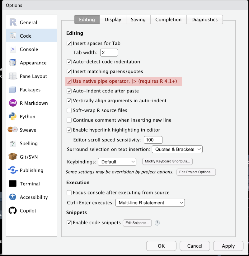
|>) or the magrittr pipe (%>%). These options can be set globally with Tools > Global Options or for a specific project with Tools > Project Options.NB: you don’t need to entirely adopt either style!
2.2.1 Reading in Data (again!)
Before we look in more detail at the data manipulation techniques which come with the dplyr package, we should look again at reading data. The readr package comes with modifications to the base R methods for reading in csv and similar files. readr includes the function read_csv (note the use of an underscore rather than dots, as in the base R function).
vowels <- read_csv(here('data', 'qb_vowels.csv'))Rows: 26331 Columns: 14
── Column specification ────────────────────────────────────────────────────────
Delimiter: ","
chr (7): speaker, vowel, participant_age_category, participant_gender, parti...
dbl (7): F1_50, F2_50, word_freq, time, vowel_duration, articulation_rate, a...
ℹ Use `spec()` to retrieve the full column specification for this data.
ℹ Specify the column types or set `show_col_types = FALSE` to quiet this message.One great advantage of read_csv is that the output tells us something about the way R has interpreted each column of the data and the names which have been given to each column. We see how many rows and columns, what delimited the values (as we expected, ","), we also see what type of data R thinks these columns contain. So, chr means text strings. These are mostly participant metadata, such as their gender or ethnic background. We also see dbl columns. These contain numerical data.2
Another change between read.csv() and read_csv() is that the data is now a ‘tibble’ rather than a base R data frame. For current purposes, you don’t need to worry about this distinction. All of the base R methods we introduced above work with tibbles and with data frames.
For more information on importing data see the relevant chapter of R for Data Science.
In the output of read_csv() above, F1_50 is listed as a column
Therefore it contains
2.2.2 Some dplyr Verbs
What are the main dplyr verbs?
If we want to filter a data frame, we use filter(). The first argument to filter() is a data frame. This argument is usually filled by the use of a pipe function (i.e., the filter() function usually appears within a pipe). The remaining arguments are a series of logical statements which say which rows you want to keep and which you want to remove. By ‘logical’ recall that we mean TRUE or FALSE. Rows which produce TRUE will be kept, those which don’t will not.
We can put multiple filtering statements inside the filter() function. Look at this code:
vowels_filtered <- vowels |>
  filter(
    following_segment_category == "other",
    !is.na(amplitude),
    between(F1_50, 300, 1000),
    vowel_duration > 0.01 | word_freq < 1000
  )
There are four statements being used to filter. Each is on a new line, but this is a stylistic choice, rather than one required for the code to work. You don’t need to use $ with column names inside tidyverse verbs.
- The first statement uses
==. This says that we only want rows in the data frame where thefollowing_segmentcolumn has the valueother. - The second statement uses the function
is.na()to test whether theamplitudecolumn is empty or not. If a row has no value foramplitudethenis.na()producesTRUE. Sois.na(amplitude)will select the rows which have no value foramplitude. We want all the values which are not empty. So we add a!to the start of the statement. This reverses the values so thatTRUEbecomesFALSEand vice versa. This statement now removes all the rows without amplitude information. - The third statement uses a helpful function from
dplyrcalledbetween()which allows us to test whether a column’s value is between a two numbers. In this case, we want our values for theF1_50column to be between \(300\) and \(1000\). This is inclusive. That is, it includes \(300\) and \(1000\). I forget this kind of thing all the time. To check, enter?betweenin the console. - The fourth statement is made up of two smaller ones, combined with a bar (
|). The bar means ‘or’. This will beTRUEwhen either of the statements isTRUE. So, in this case, it selects rows which have avowel_durationvalue greater than \(0.01\) and rows which have aword_freqvalue less than \(1000\).3
We have seen mutate() and rename() already. mutate() is used to create new columns and to modify existing columns. The statements in a mutate() function are all of the form column_name =, with an R statement defining the values which the column will take. These can be either a single value, if you want every row of the column to have the same value (e.g. version = 1 would create a column called version which always has the value \(1\)), or a vector with a value for each row of the data frame. If you get this wrong it will look like this:
vowels |>
  mutate(
    bad_column = c(1, 2, 3, 4)
  )
Error in `mutate()`:
ℹ In argument: `bad_column = c(1, 2, 3, 4)`.
Caused by error:
! `bad_column` must be size 26331 or 1, not 4.If you want a subset of the columns, you can use select(). Here is an example:
participant_metadata <- vowels_filtered |>
  select(
    speaker,
    contains('participant_')
  ) |>
  unique()
The select() verb here has two arguments. The first is just the name speaker. This, unsurprisingly, selects the column speaker. The second, contains('participant_') uses the function contains() (also from dplyr) to pick out columns containing the string 'participant_' in their names.4 After selecting these columns, there are many duplicate rows, so we pass the result into the base R function unique() with a pipe. The result is a data frame with the meta data for each participant in the data. Look in the environment pane to see how many rows and columns there are in the data frame participant_metadata.
The relocate() function is sometimes useful with the nzilbb.vowels package and other packages where the order of the columns is important. It relocates columns within a data frame. See for instance,
We have just covered:
mutate(): the change a data frame.rename(): to change the names of existing columns.filter(): to filter the rows of a data frame.select(): to select a subset of columns of the data.relocate(): to move selected columns within a data frame.
Consider the following code. Assume that vowels has columns called F1_50 andF2_50.
vowels <- vowels |>
  rename(
    first_formant = F1_50,
    second_formant = F2_50
)- After running the code,
qb_vowelswill have a column calledfirst_formant: . - After running the code,
qb_vowelswill have a column calledF2 _50: .
2.2.3 Grouped Data
Another advantage of dplyr is that the same functions work for grouped data and ungrouped data. What is grouped data? It is data in which a group structure is defined by one or more of the columns.
This is most clear by example. In the data frame we have been looking at, we have a series of readings for a collection of speakers. There are only 77 speakers in the data frame, from which we get more than 20,000 rows. What if we want to get the mean values of these observations for each speaker? That is, we treat the data frame as one which is grouped by speaker.
In order to group data we use the group_by() function. In order to remove groups we use the ungroup() function. Let’s see this in action:
vowels_filtered <- vowels_filtered |>
  group_by(speaker) |>
  mutate(
    mean_F1 = mean(F1_50),
    mean_amplitude = mean(amplitude)
  ) |>
  ungroup()
The above code groups the data, then uses mutate(), in the same way as we did above, to create two new columns. These use the mean() function, from base R, to calculate the mean value for each speaker. Have a look at the data, using one of the methods for accessing data we discussed above, to convince yourself that each speaker is given a different mean value. The same points apply to amplitude. Note, by the way, that the mean() function returns NA if there are any NA values in the column. This is a common issue. If you see NA when you expect a sensible mean, you can add na.rm = TRUE to the arguments of mean() or filter out any rows with missing information before you apply mean().
Sometimes we want summary information for each group. In this case, it is useful to have a data frame with a single row for each group. To do this, we use summarise rather than mutate. We can combine the output of the code block we have just looked at with the participant metadata as follows:
vowels_summary <- vowels_filtered |>
  group_by(speaker) |>
  summarise(
    n = n(),
    mean_F1 = mean(F1_50),
    mean_amplitude = mean(amplitude),
    gender = first(participant_gender),
    age_category = first(participant_age_category)
  )

vowels_summary |>
  head()
# A tibble: 6 × 6
speaker n mean_F1 mean_amplitude gender age_category
<chr> <int> <dbl> <dbl> <chr> <chr>
1 QB_NZ_F_138 86 572. 61.0 F 18-25
2 QB_NZ_F_161 273 433. 76.9 F 18-25
3 QB_NZ_F_169 100 461. 69.5 F 66-75
4 QB_NZ_F_195 138 558. 65.9 F 26-35
5 QB_NZ_F_200 259 521. 63.7 F 56-65
6 QB_NZ_F_213 218 513. 69.4 F 66-75 The code above has two statements. We create a data frame called vowels_summary, which uses summarise() instead of mutate(). The second statement outputs the first six rows of vowels_summary using the head() function. Each row is for a different speaker and each column is defined by the grouping structure and summarise(). There is a column for each group (in this case just speaker), and then one for each argument to summarise(). The first, n, uses the n() function to count how many rows there are for each speaker. The second and third columns contain the mean value for the speaker for two variables. We then use the function first() to pull out the first value for the speaker for a given column. This is very useful in cases when every row for the speaker should have the same value. In this case, the speaker’s age category, for instance, does not change within a single recording so we can safely just take the first value for participant_age_category for each speaker.
Consider the following code:
vowels_summary <- vowels |>
  group_by(participant_gender, vowel) |>
  summarise(
    n = n(),
    F1_50 = mean(F1_50),
    any_loud = any(amplitude > 85, na.rm = TRUE),
    all_loud = all(amplitude > 85, na.rm = TRUE)
)- There are 11 vowels and 2 genders in
vowels. How many rows are there invowel_summary?
n() in this code?
- Experiment with the
mean()functiona. What does the function output if it getsNAvalues (e.g.mean(c(1, 2, 3, NA, 5)))?
2.2.4 Pivoting data
This is a quick note on pivot_longer() and pivot_wider() from the tidyr package. These enable you to change the repesentation of the data in your data frame so that more information is carried in rows (i.e., you have more rows, therefore a ‘longer’ data frame), or columns (i.e., you have more columns, therefore a ‘wider’ data frame).
Pivoting is tied up with the idea of a ‘tidy’ data set, which I haven’t written much about in this chapter so far. The basic idea is that we want data where each row is an observation and each column is a variable. Pivoting is useful for getting to this point (and that’s why the pivot function are in a package called tidyr).
For our purposes, it’s worth noticing that sometimes we need to shift between different ideas of what our observations are. Sometimes they might be individual formant readings, sometimes they might be individual vowel tokens, and sometimes they might be speakers. Pivoting is useful for shifting between these representations of the data.
Here’s an example of a shift to a ‘longer’ formant.
## Split F1_midpoint and F2_midpoint into distinct rows (now a 'formant reading'
## is our observation rather than an individual vowel token.) That is, make the
## data 'longer'.
vowels_long <- vowels_filtered |>
  pivot_longer(
    # Which columns do we want to 'lengthen'?
    cols = c(F1_50, F2_50),
    # What do we want to name the column which identifies the kind of formant
    # reading?
    names_to = "formant_type",
    # What do we want to name the column containing the formant values?
    values_to = "formant_value"
  )

head(vowels_long |> select(speaker, vowel, formant_type, formant_value))
# A tibble: 6 × 4
speaker vowel formant_type formant_value
<chr> <chr> <chr> <dbl>
1 QB_NZ_F_281 DRESS F1_50 440
2 QB_NZ_F_281 DRESS F2_50 2320
3 QB_NZ_F_281 NURSE F1_50 434
4 QB_NZ_F_281 NURSE F2_50 1795
5 QB_NZ_F_281 START F1_50 851
6 QB_NZ_F_281 START F2_50 1810The above code moves us from a data frame with 17240 to one with 34480 rows. The ‘observations’ are now individual formant readings.
Now look at an example where we pivot ‘wider’:
# What is we want a single row for each speaker, with their mean value for each
# vowel as columns.
vowels_wide <- vowels_filtered |>
  # Select only relevant data
  select(
    speaker, vowel, F1_50, F2_50,
    contains(match = "participant_")
  ) |>
  pivot_wider(
    # Column names come from 'vowel' column
    names_from = vowel,
    # Values come from both midpoint columns
    values_from = c(F1_50, F2_50),
    # We aggregate using the `mean` function if there is more than
    # one value for each cell of the table. i.e., the `F1_midpoint_DRESS`
    # column will end up with the mean F1 value across *all* the speakers tokens
    # of DRESS.
    values_fn = mean
  )

head(vowels_wide |> select(speaker, matches("F1|F2")))
# A tibble: 6 × 23
speaker F1_50_DRESS F1_50_NURSE F1_50_START F1_50_STRUT F1_50_GOOSE
<chr> <dbl> <dbl> <dbl> <dbl> <dbl>
1 QB_NZ_F_281 439. 417 858. 606. 389.
2 QB_NZ_F_377 396. 372. 771. 646. 388
3 QB_NZ_F_432 439. 443. 886. 653. 394.
4 QB_NZ_F_449 439 443. 847. 692. 467.
5 QB_NZ_F_470 495. 524 926. 816 380
6 QB_NZ_F_478 408. 403. 804. 639. 381.
# ℹ 17 more variables: F1_50_FLEECE <dbl>, F1_50_TRAP <dbl>, F1_50_LOT <dbl>,
# F1_50_FOOT <dbl>, F1_50_KIT <dbl>, F1_50_THOUGHT <dbl>, F2_50_DRESS <dbl>,
# F2_50_NURSE <dbl>, F2_50_START <dbl>, F2_50_STRUT <dbl>, F2_50_GOOSE <dbl>,
# F2_50_FLEECE <dbl>, F2_50_TRAP <dbl>, F2_50_LOT <dbl>, F2_50_FOOT <dbl>,
# F2_50_KIT <dbl>, F2_50_THOUGHT <dbl>Here we have switched from a representation of the data in terms of vowel tokens to one in terms of speakers. We have aggregated the data so that each cell contains the mean value for each speaker of each vowel and formant reading. For instance, there is now a column called F1_50_DRESS, which contains the mean midpoint first formant reading for each speaker’s dress vowel.
2.3 Further Resources
- For a fuller introduction to data transformation in the tidyverse see R for Data Science
- For a discussion more focused on linguistics see the second chapter of Winter (2019).
- For a discussion of the differences between base R and
dplyrapproaches to data processing see this vignette fromdplyr.
There are some slight differences. If you are interested see the relevant section of Advanced R↩︎
A
dblis a double length floating point number… Just think a number which can have a decimal point. Computers are, obviously, finite systems. Numbers are not (well… you could become a strict finitist I suppose). The technicalities of representing numbers on computers are very interesting, but we will avoid them where we can!↩︎This juggling of ‘true’ and ‘false’ is a bit of formal logic and make take a while to get your head around if you haven’t come across formal logic before.↩︎
The documentation for
select()covers a bunch of other helper functions likecontains(). As usual, just type?selectin the console.↩︎