Word Frequency
LaBB-CAT can generate frequency data about your corpus; i.e. count the number of tokens of each word (type) that appears in you transcripts. LaBB-CAT can both
- Generate a list of word types with the token count of each type, and
- Tag each token in the corpus with its frequency (token count)
To do this:
- Select the word layers menu option.
You will see a list of word layers. - The row of headers at the top of the list is also a form you can fill in to add a new layer.
Fill in the following details:- Layer ID:
frequency - Type: Number
- Alignment: None
- Manager: Frequency Layer Manager
- Generate: Always
- Description:
Count of tokens of the same type across all corpora.
- Layer ID:
- Press the New button to add the layer.
- You will see the layer configuration form. Fill it in with the following details:
- Summary: Raw Count
- Layer to summarize: orthography
- Scope of Summary: Database
- Main participants only: ticked
- Participants: unticked
- Filter Layer: unticked
- Word pairs: unticked
- WordPause Markers: (Leave this box empty)
- Transcript types: If you have a word-list or reading trascript type, un-tick it to ensure that your readings don’t make certain words over-represented in the frequency counts.
- Annotate tokens: ticked
If you want more information about what these options mean, check the online help page by clicking the question-mark icon at the top right of the page. This will provide information about how to break down counts by corpus, by speaker, etc.
- Press Save
- Press Regenerate
You will see a progress bar moving across the page while the counts are being generated. When it is finished, you will see a message saying Layer complete.
Now each word in each transcript is annotated with the count of the number of instances of that word with the corpus of the transcript. To see what that looks like:
- Select the transcripts menu option.
- Click the name of the first transcript in the list.
- Tick the frequency layer.
When the transcript reloads, you will see that above each word is a number. That number is the number of times that word appears in the transcript’s corpus. e.g. if the word “and” has 1743 above it, that means that the word “and” appears in the corpus 1743 times.

The new word tags are searchable and exportable into CSV results files, just like any other annotations; If you do any search, the CSV Export options dropdown now contains a frequency checkbox that allows you to include the word frequency of the matches as a column in the CSV file.
If you have already exported the CSV results previously, and want to insert frequencies into the existing CSV file, you can do this by using the uploads → insert data option.
The Frequency Layer Manager also keeps a word-list with token counts for each corpus:
- Select the layer managers menu option.
- On the Frequency Layer Manager row, press the Extensions button.
- (If you have multiple Frequency Layer Manager layers, you will have to select the layer you’re after from the list, and then press Select. If you have only one Frequency Layer Manager layer, this step is not necessary.)
- Press Export
- Save and open the resulting CSV file.
You will see an alphabetical list of all the distinct word types in your corpus, and next to each, a count of the number of tokens of that type.
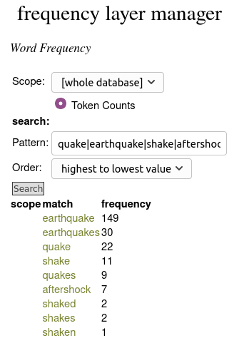
This page can also be used to search for target words and list their frequencies directly on the page.
The steps above will give you basic word-form counts across all your data. The Frequency Layer Manager can be used to calculate other frequencies too:
- Stem/lemma frequencies can be computed if you have tagged each word token with its stem (e.g. using the Porter Stemmer Layer Manager or the CELEX Layer Manager); to do this, specify the stem or lemma layer generated by the other layer manager as the Layer to Summarize for the Frequency Layer Manager.
- If you have several sub-corpora in your database, you can get frequencies by corpus, by selecting “Corpus” as the Scope of Summary.
- Similarly you can get frequencies by speaker, to get information of each speaker’s vocabulary use, by selecting “Speaker” as the Scope of Summary.
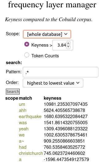
- You can compare frequencies in your corpus against a reference corpus, in order to identify unusually frequent or infrequent words, by selecting Keyness as the Summary option, and then selecting a reference corpus.
For this option to work, you must have frequencies from a reference corpus loaded as a dictionary into LaBB-CAT; e.g. if you have installed the CELEX Layer Manager, this includes word-form and lemma frequencies from reference corpora.
Word Pair Frequency List
If you want word tokens tagged with their individual frequencies, and also want a word-pair frequency list, simply tick the Word Pairs option when you create the word layer to get an extra word-pair list.
This does not tag word tokens with bigram frequencies, so you can’t see the word-pair frequencies in transcript, nor extract them as part of search results files. But it does keep a list of frequencies that can be downloaded separately.
To access the word pair frequency list:
- Select the layer managers menu option.
- On the Frequency Layer ManagerI row, press the Extensions button.
- (If you have multiple Frequency Layer Manager layers, you will have to select the layer you’re after from the list, and then click Select. If you have only one Frequency Layer Manager layer, this step is not necessary.)
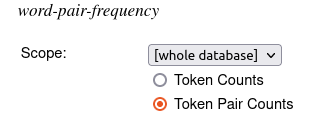
- Select the Token Pair Counts option:
- Press Export
- Save and open the resulting CSV file; you will see there are three columns:
- Word1 - the first word in the pair
- Word2 - the second word in the pair
- 0 words between - the number of times Word1 is immediately followed by Word2
Note that when configuring the layer, next to the Word Pairs checkbox, there’s a dropdown box with ‘adjacent’ selected by default. This option lets you get frequencies for word pairs that are further apart. e.g. if you select the ‘within 1 word’ option, then in addition to the Word1, Word2, and 0 words between columns in the CSV file, you’ll also get a 1 words between column, containing the number of times Word1 is followed by Word2 with one intervening word.
N-gram Annotations
If you not only want bigram frequencies in a list, but you also want to token pairs themselves annotated with that bigram’s frequency, or you’re interested in frequencies of trigrams or larger word clusters, you can use the Frequency Layer Manager to tag multiple words with their n-gram frequencies.
For example, to tag bigrams with their frequencies:
- Select the phrase layers option on the menu (because instead of tagging individual word tokens, we’re going to create annotations that cover multiple words within the same speaker turn).
- Create a layer with the following characteristics
- Layer ID:
bigram - Type: Number
- Alignment: Intervals
- Manager: Frequency Layer Manager
- Generate: Always
- Description:
Bigram frequencies
- Layer ID:
- On the configuration page, use the following settings:
- Summary: Raw Count
- Layer to Summarize: orthography (unless you’re interested in combinations of stems/lemmas, in which case select your stem/lemma layer)
- Scope of Summary: Database
- Main participants only: ticked (unless you want to include interviewer speech or other incidental speakers)
- Participants: unticked
- Filter Layer: unticked
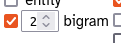
- N-gram: ticked, and leave the bigram option selected
- Under Transcript Types you may want to un-tick ‘word list’ or ‘reading’ transcript types, if you have them, in order to only include spontaneous speech
- Annotate Tokens: ticked
- Press Save
- Press Regenerate
Once the annotation layer has been generated, if you open a transcript and tick the bigram layer you just created, you’ll see that each pair of words has been annotated with a number; the frequency of that bigram:

For example, you can see that the bigram “first one” appears 7 times in this corpus.
You can see that each word token is covered by two annotations; for when it’s the first word in the bigram, and for when it’s the second word in the bigram. For example, the token “one” above is at the beginning of the “one being” bigram (labelled “1”), and at the end of the “first one” bigram (labelled “7”).
When you extract bigram frequency annotations in search results, you can extract both of these frequencies; when you do a search, expand the CSV Export options to select layers, and tick the bigram layer, you will see a box with a number appear. Enter 2 in the box to extract two bigram annotations per match.
The resulting CSV file will have two columns for the bigram layer:
Target bigram 1- the chronologically first bigram the target is part of (i.e. where it is the second word).Target bigram 2- the chronologically second bigram the target is part of (i.e. where it is the first word).
(You will also have Target bigram 1 start, Target bigram 1 end, Target bigram 2 start, and Target bigram 2 end columns; these will contain the start and end times of the bigram annotations, but only if the words have been aligned.)